
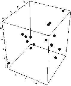
3D Scatter Plot of data read from a file
November 29, 2007 Posted by Emre S. Tasci
We’re soon going to need this information when playing a game called clustering so, it’s handy to have this around.
Suppose that the data belong to the positions of some number of particles given in Cartesian coordinates. The file (let’s assume it resides in the root of the d drive, having the name "lol1.txt") looks something similar to this:
4.455 3.302 6.858
4.909 4.997 5.447
6.898 8.167 7.083
8.589 5.387 4.953
5.222 3.425 5.684
8.568 6.414 6.037
6.348 2.604 5.356
7.584 7.778 2.810
8.544 9.546 9.098
3.724 5.381 4.913
6.561 8.245 6.550
9.231 5.904 2.066
9.578 6.581 3.521
2.239 1.841 1.004
7.703 5.159 5.714
4.411 6.937 2.433
First, let’s try it in Mathematica:
m=OpenRead["d:\lol1.txt"];
k= ReadList[m,Number];
Close[m];
(k =Partition[k,3]) // TableForm
(* And you can definitely Plot it too *)
<<Graphics`Graphics3D`
PlotStyle->{{PointSize[0.04],GrayLevel[0.09]}}]
Actually, I just copied the above code from a previous entry (but I had updated it just yesterday, so it is still fresh) the output graph will look like this:
It is not that much practical to change the view angle (or most probably I don’t know how to do it) using Mathematica…
You can, for example, try something like this:
For[i=1,i<10,i+=1,ScatterPlot3D[k,PlotStyle->{{PointSize[0.04],GrayLevel[0.09]}},ViewPoint->{-2,i,2},AxesLabel->{"x","y","z"}]]
Or, if you have Mathcad with you, you can do this much simpler and more enjoyable way, too (but be warned, if I believed that Mathcad was superior to Mathematica, I would have a category for Mathcad instead of Mathematica category I’m having now – Mathcad actually from time to time makes you want to bite the keyboard! ;)! I decided to use Mathcad to visualize my scatter pattern and at once realized that, it has been nearly 5 years since I last used it. My favourite package used to be MapleV but -in my opinion- the Waterloo guys just tore it down when they switched the code language to Java. That was when our ways parted. Maple had nice graphics feature, too. So, if you’re using please send me your version of this entry… So, back to Mathcad:
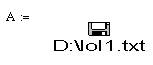
First, from the "Insert…" menu, select "Component", then "File Read or Write" as the type and then select "Read from file". Browse to the designated file and make sure that "Use comma as decimal symbol" is unchecked since we’re using "." for the seperator. By the way, I’m using Mathcad2001 so it may (may?! more like surely!) be a little bit different about the options…
Attach a symbol to this file, say A so that now we have smt like:
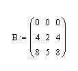
Now, just for the fun of it, define another set like:
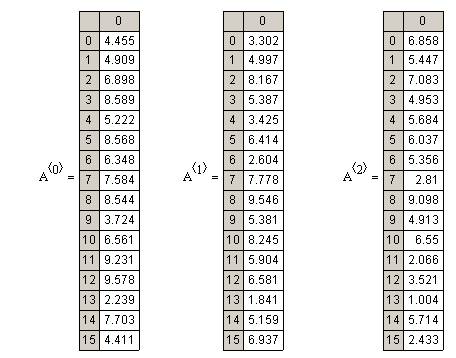
You may also check your data if you want:
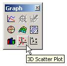
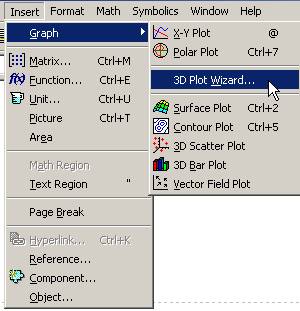
Now define a 3D Scatter Plot either from the Graph Pallette, or more preferably from the Insert menu:
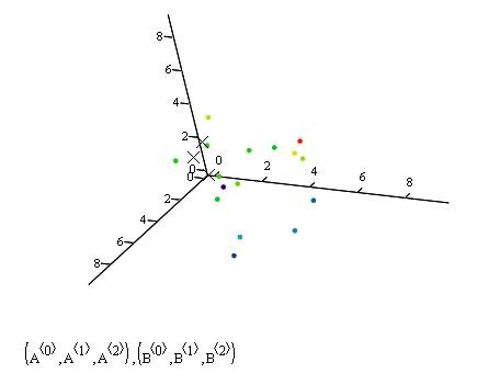
Fill in the data section of the plot as (A<0>,A<1>,A<2>),(B<0>,B<1>,B<2>) and it’s all yours!
With mathcad I was able to rotate the graph whichever way I wanted and also could easily include data from different sources (like the A and B in the example) and plot them any way I wanted to. Here are the snapshots from a more "cute" plot with 500 data points:
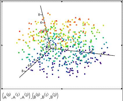
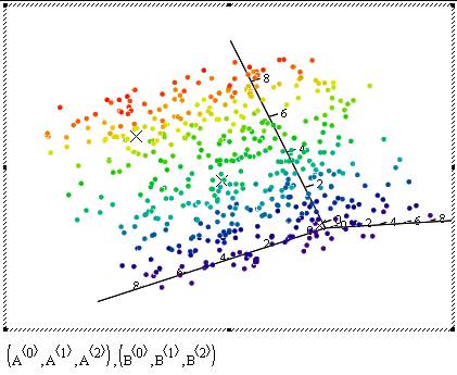
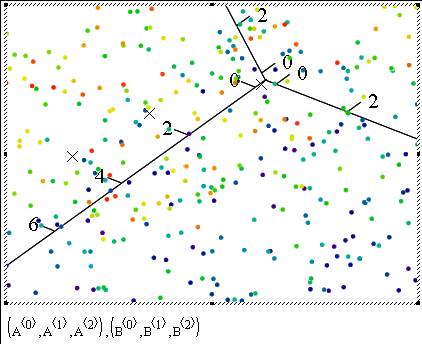
Hint for our game to be announced: Let’s call the little points in the plot as data’s and the Xs as "K-Means"
Splendid news from homeland..
Posted by Emre S. Tasci
Yesterday, I received great news from my dear former supervisor, Prof. Erkoç, that my Generation and Simulations of Nanostructures of Cage Structures titled Ph.D. thesis has been selected as one of the thesis of the year by METU Mustafa Parlar Foundation, the most distinctive and prestigious award a METU thesis can receive!
I would like to express my gratitude to Prof. Erkoç, all my friends and the physics department for the great days I’ve enjoyed for the seven years I was in METU. I will always cherish the memories… I hope, here in my new home S&C/MSE@TUDelft, I will live up to the expectations.
.jpg)
With Prof. Åakir Erkoç sitting in the front row, rest of our team is (from left to right):
O.BarıŠMalcıoÄlu, Hande Üstünel, E. Deniz ÇalıÅır Tekin, Nazım Dugan, Emre S. TaÅcı, Rengin Peköz
Bayesian Probabilities & Inference – Another example
November 27, 2007 Posted by Emre S. Tasci
Yesterday, I told my battalion-buddy, Andy about the pregnancy example and, he recalled another example, with the shuffling of the three cups and a ball in one of them. The situation is proposed like this:
The dealer puts the ball in one of the cups and shuffles it so fast that at one point you lose the track and absolutely have no idea which cup has the ball. So, you pick a cup randomly (let’s say the first cup) but for the moment, don’t look inside. At this point, the dealer says, he will remove one of the remaining two cups and he guarantees you that, the one he removes does not have the ball. He even bestows you the opportunity to change your mind and pick the other one if you like. The question is this: Should you
a) Stick to the one you’ve selected or,
b) Switch to the other one or,
c) (a) or (b) – what does it matter?
Today, while I was studying MacKay’s book Theory, Inference, and Learning Algorithms, I came upon to the same example and couldn’t refrain myself from including it on this blog.
First, let’s solve the problem with simple notation. Let’s say that, initially we have picked the first cup, the probability that this cup has the ball is 1/3. There are two possibilities: Whether in reality the 1st cup has the ball indeed, or not.
i) 1st cup has the ball (1/3 of all the times): With this situation, it doesn’t matter which of the two cups remaining is removed.
ii) 1st cup doesn’t have the ball (2/3 of all the times): This time, the dealer removes the one, and the remaining cup has the ball.
So, to summarize, left with the two cups, there’s a 1/3 probability that the ball is within the cup we have chosen in the beginning while there’s the 2/3 probability that the ball is within the other cup. So, switching is the advantegous (did I spell it correctly? Don’t think so.. ) / To put it in other words: option (b) must be preffered to option (a) and actually, option (c) is wrong.
Now, let’s compute the same thing with the formal notations:
Let Hi be define the situation that the ball is in cup i. D denotes the removed cup (either 2 or 3). Now, initially the ball can be in any of the three cups with equal probabilities so
![Formula: % MathType!MTEF!2!1!+-<br />
% feaafiart1ev1aaatCvAUfeBSjuyZL2yd9gzLbvyNv2CaerbuLwBLn<br />
% hiov2DGi1BTfMBaeXatLxBI9gBaerbd9wDYLwzYbItLDharqqtubsr<br />
% 4rNCHbGeaGqiVu0Je9sqqrpepC0xbbL8F4rqqrFfpeea0xe9Lq-Jc9<br />
% vqaqpepm0xbba9pwe9Q8fs0-yqaqpepae9pg0FirpepeKkFr0xfr-x<br />
% fr-xb9adbaqaaeGaciGaaiaabeqaamaabaabaaGcbaGaamiuamaabm<br />
% aabaGaamisamaaBaaaleaacaaIXaaabeaaaOGaayjkaiaawMcaaiab<br />
% g2da9iaadcfadaqadaqaaiaadIeadaWgaaWcbaGaaGymaaqabaaaki<br />
% aawIcacaGLPaaacqGH9aqpcaWGqbWaaeWaaeaacaWGibWaaSbaaSqa<br />
% aiaaigdaaeqaaaGccaGLOaGaayzkaaGaeyypa0ZaaSqaaSqaaiaaig<br />
% daaeaacaaIZaaaaaaa!46E7!<br />
\[<br />
P\left( {H_1 } \right) = P\left( {H_1 } \right) = P\left( {H_1 } \right) = \tfrac{1}<br />
{3}<br />
\]<br />](../latex_cache/ad1a07b9d6fc3e0f068887aff30c0ec3.png)
Now, since we have selected the 1st cup, either 2nd or the 3rd cup will be removed. And we have three cases for the ball position:
![Formula: % MathType!MTEF!2!1!+-
% feaafiart1ev1aaatCvAUfeBSjuyZL2yd9gzLbvyNv2CaerbuLwBLn
% hiov2DGi1BTfMBaeXatLxBI9gBaerbd9wDYLwzYbItLDharqqtubsr
% 4rNCHbGeaGqiVu0Je9sqqrpepC0xbbL8F4rqqrFfpeea0xe9Lq-Jc9
% vqaqpepm0xbba9pwe9Q8fs0-yqaqpepae9pg0FirpepeKkFr0xfr-x
% fr-xb9adbaqaaeGaciGaaiaabeqaamaabaabaaGcbaWaaqGaaeaafa
% qabeGabaaabaGaamiuaiaacIcacaWGebGaeyypa0JaaGOmaiaacYha
% caWGibWaaSbaaSqaaiaaigdaaeqaaOGaaiykaiabg2da9maaleaale
% aacaaIXaaabaGaaGOmaaaaaOqaaiaadcfacaGGOaGaamiraiabg2da
% 9iaaiodacaGG8bGaamisamaaBaaaleaacaaIXaaabeaakiaacMcacq
% GH9aqpdaWcbaWcbaGaaGymaaqaaiaaikdaaaaaaaGccaGLiWoafaqa
% beGabaaabaGaamiuaiaacIcacaWGebGaeyypa0JaaGOmaiaacYhaca
% WGibWaaSbaaSqaaiaaikdaaeqaaOGaaiykaiabg2da9iaaicdaaeaa
% caWGqbGaaiikaiaadseacqGH9aqpcaaIZaGaaiiFaiaadIeadaWgaa
% WcbaGaaGOmaaqabaGccaGGPaGaeyypa0JaaGymaaaadaabbaqaauaa
% beqaceaaaeaacaWGqbGaaiikaiaadseacqGH9aqpcaaIYaGaaiiFai
% aadIeadaWgaaWcbaGaaG4maaqabaGccaGGPaGaeyypa0JaaGymaaqa
% aiaadcfacaGGOaGaamiraiabg2da9iaaiodacaGG8bGaamisamaaBa
% aaleaacaaIZaaabeaakiaacMcacqGH9aqpcaaIWaaaaaGaay5bSdaa
% aa!7259!
\[
\left. {\begin{array}{*{20}c}
{P(D = 2|H_1 ) = \tfrac{1}
{2}} \\
{P(D = 3|H_1 ) = \tfrac{1}
{2}} \\
\end{array} } \right|\begin{array}{*{20}c}
{P(D = 2|H_2 ) = 0} \\
{P(D = 3|H_2 ) = 1} \\
\end{array} \left| {\begin{array}{*{20}c}
{P(D = 2|H_3 ) = 1} \\
{P(D = 3|H_3 ) = 0} \\
\end{array} } \right.
\]](../latex_cache/4fc864c6872eb6452e816e7eadc00fdd.png)
The first column represents that the ball is in our selected cup, so it doesn’t matter which of the remaining cups the dealer will remove. Each of the remaining cup has the same probability to be removed which is 0.5. The second column is the situation when the ball is in the second cup. Since it is in the second cup, the dealer will be forced to remove the third cup (ie P(D=3|H2)=1 ).Third column is similar to the second column.
Let’s suppose that, the dealer removed the third cup. With the 3rd cup removed, the probability that the ball is in the i. cup is given by: (remember that Hi represents the situation that the ball is in the i. cup)
![Formula: % MathType!MTEF!2!1!+-
% feaafiart1ev1aaatCvAUfeBSjuyZL2yd9gzLbvyNv2CaerbuLwBLn
% hiov2DGi1BTfMBaeXatLxBI9gBaerbd9wDYLwzYbItLDharqqtubsr
% 4rNCHbGeaGqiVu0Je9sqqrpepC0xbbL8F4rqqrFfpeea0xe9Lq-Jc9
% vqaqpepm0xbba9pwe9Q8fs0-yqaqpepae9pg0FirpepeKkFr0xfr-x
% fr-xb9adbaqaaeGaciGaaiaabeqaamaabaabaaGcbaGaamiuamaabm
% aabaGaamisamaaBaaaleaacaWGPbaabeaakiaacYhacaWGebGaeyyp
% a0JaaG4maaGaayjkaiaawMcaaiabg2da9maalaaabaGaamiuamaabm
% aabaGaamiraiabg2da9iaaiodacaGG8bGaamisamaaBaaaleaacaWG
% PbaabeaaaOGaayjkaiaawMcaaiaadcfadaqadaqaaiaadIeadaWgaa
% WcbaGaamyAaaqabaaakiaawIcacaGLPaaaaeaacaWGqbWaaeWaaeaa
% caWGebGaeyypa0JaaG4maaGaayjkaiaawMcaaaaaaaa!4FF2!
\[
P\left( {H_i |D = 3} \right) = \frac{{P\left( {D = 3|H_i } \right)P\left( {H_i } \right)}}
{{P\left( {D = 3} \right)}}
\]](../latex_cache/34a6b3faa776ca6104636141b00e21d8.png)
![Formula: % MathType!MTEF!2!1!+-
% feaafiart1ev1aaatCvAUfeBSjuyZL2yd9gzLbvyNv2CaerbuLwBLn
% hiov2DGi1BTfMBaeXatLxBI9gBaerbd9wDYLwzYbItLDharqqtubsr
% 4rNCHbGeaGqiVu0Je9sqqrpepC0xbbL8F4rqqrFfpeea0xe9Lq-Jc9
% vqaqpepm0xbba9pwe9Q8fs0-yqaqpepae9pg0FirpepeKkFr0xfr-x
% fr-xb9adbaqaaeGaciGaaiaabeqaamaabaabaaGcbaWaaqGaaeaaca
% WGqbWaaeWaaeaacaWGibWaaSbaaSqaaiaaigdaaeqaaOGaaiiFaiaa
% dseacqGH9aqpcaaIZaaacaGLOaGaayzkaaGaeyypa0ZaaSaaaeaada
% WcbaWcbaGaaGymaaqaaiaaikdaaaGccqGHflY1daWcbaWcbaGaaGym
% aaqaaiaaiodaaaaakeaacaWGqbWaaeWaaeaacaWGebGaeyypa0JaaG
% 4maaGaayjkaiaawMcaaaaaaiaawIa7aiaadcfadaqadaqaaiaadIea
% daWgaaWcbaGaaGOmaaqabaGccaGG8bGaamiraiabg2da9iaaiodaai
% aawIcacaGLPaaacqGH9aqpdaWcaaqaaiaaigdacqGHflY1daWcbaWc
% baGaaGymaaqaaiaaiodaaaaakeaacaWGqbWaaeWaaeaacaWGebGaey
% ypa0JaaG4maaGaayjkaiaawMcaaaaadaabbaqaaiaadcfadaqadaqa
% aiaadIeadaWgaaWcbaGaaGOmaaqabaGccaGG8bGaamiraiabg2da9i
% aaiodaaiaawIcacaGLPaaacqGH9aqpdaWcaaqaaiaaicdacqGHflY1
% daWcbaWcbaGaaGymaaqaaiaaiodaaaaakeaacaWGqbWaaeWaaeaaca
% WGebGaeyypa0JaaG4maaGaayjkaiaawMcaaaaaaiaawEa7aaaa!70DB!
\[
\left. {P\left( {H_1 |D = 3} \right) = \frac{{\tfrac{1}
{2} \cdot \tfrac{1}
{3}}}
{{P\left( {D = 3} \right)}}} \right|P\left( {H_2 |D = 3} \right) = \frac{{1 \cdot \tfrac{1}
{3}}}
{{P\left( {D = 3} \right)}}\left| {P\left( {H_2 |D = 3} \right) = \frac{{0 \cdot \tfrac{1}
{3}}}
{{P\left( {D = 3} \right)}}} \right.
\]](../latex_cache/d28519eef1c192c02bd65d0840ec790b.png)
for our purposes, P(D=3) is not relevant, because we are looking for the comparison of the first two probabilities (P(D=3) = 0.5, by the way since it is either D=2 or D=3).
![Formula: % MathType!MTEF!2!1!+-
% feaafiart1ev1aaatCvAUfeBSjuyZL2yd9gzLbvyNv2CaerbuLwBLn
% hiov2DGi1BTfMBaeXatLxBI9gBaerbd9wDYLwzYbItLDharqqtubsr
% 4rNCHbGeaGqiVu0Je9sqqrpepC0xbbL8F4rqqrFfpeea0xe9Lq-Jc9
% vqaqpepm0xbba9pwe9Q8fs0-yqaqpepae9pg0FirpepeKkFr0xfr-x
% fr-xb9adbaqaaeGaciGaaiaabeqaamaabaabaaGcbaWaaSaaaeaaca
% WGqbWaaeWaaeaacaWGibWaaSbaaSqaaiaaigdaaeqaaOGaaiiFaiaa
% dseacqGH9aqpcaaIZaaacaGLOaGaayzkaaaabaGaamiuamaabmaaba
% GaamisamaaBaaaleaacaaIYaaabeaakiaacYhacaWGebGaeyypa0Ja
% aG4maaGaayjkaiaawMcaaaaacqGH9aqpdaWcaaqaaiaaigdaaeaaca
% aIYaaaaaaa!47DB!
\[
\frac{{P\left( {H_1 |D = 3} \right)}}
{{P\left( {H_2 |D = 3} \right)}} = \frac{1}
{2}
\]](../latex_cache/b0d88841dfc32e38f97cc991beb7a930.png)
meaning that it is 2 times more likely that the ball is in the other cup than the one we initially had selected.
Like John, Jo’s funny boyfriend in the previous bayesian example, used in context to show the unlikeliness of the "presumed" logical derivation, MacKay introduces the concept of one million cups instead of the three. Suppose you have selected one cup among the one million cups. Then, the dealer removes 999,998 cups and you’re left with the one you’ve initially chosen and the 432,238th cup. Would you now switch, or stick to the one you had chosen?
Lewis “Powering the Planet” MRS Bulletin 32 808 2007
Posted by Emre S. Tasci
Powering the Planet / Nathan S. Lewis
MRS Bulletin 32 808 2007
(Recommended by Prof. Thijsse)
This article is an edited transcript based on the plenary presentation given by Nathan S. Lewis (California Institute of Technology) on April 11, 2007, at the Materials Research Society Spring Meeting in San Fransisco.
- Richard Smalley’s collaborator.
- The problem is not the extinction of fossil based fuels, they will be available for the future (roughly 50-150 years for oil / 200-600 years of natural gas / 2000 years of coal). "This does not even include the methane clathrates, off the continental shelves, which are estimated to exist in comparable quantities to all of the oil, coal and gas on our planet combined."
- The article focuses on the planet in the year 2050:
I chose 2050 for two reasons. First, achieving results in the energy industry is a much longer-term endeavor than, say, achieving results in the information technology business. In IT, for example, you can build a Web site and only a few years later become a Google. If you build a coalfired power plant, however, it will take about 40 years to pay itself off and deliver a reasonable return on investment. The energy infrastructure that we build in the next 10 years, therefore, is going to determine, by and large, what our planet’s energy mix is going to look like in 2050. The second reason for choosing 2050 is that today’s population wants to know what our planet’s energy picture is going to look like within a timeframe meaningful to them—the next 30 to 40 years.
- The real problem is the CO2 emission. If we stop emitting carbondioxide as of this moment, it will be about 350 ppm by 2050. Even 550 ppm rate looks pretty hard to obtain. "We do not know, except through climate models, what the implications of driving the atmospheric CO2 concentrations to any of these levels will be. There are about six major climate models, all differing from each other in detail."
- What can be done?
1 – Nuclear Power – Insufficient.
2 – Carbon sequestration – Very insufficient. "The U.S. department of Energy is doing work on carbon sequestration, with the goal of creating 1 gigaton of storage by 2025 and 4 gigatons total by 2050. Since the United State’s annual carbon emissions are 1.5 gigaton per year, the total DOE goal for 50 years from now is commensurate with a few years’ worth of current emissions.
3 – Renewable Carbon-Neutral Energy Sources – Highly insufficient. Not the time, nor the areas are available for this to work. But we should head to the sun. "To put that another way, more energy from the sun hits the earth in one hour than all of the energy consumed on our planet in an entire year." Also there is some debate about using geothermal energy but the the low temperature difference that will practically let us extract much less than a few terrawats sustainably over the 11.6 TW of sustainable global heat energy. - Solar cells / sun energy collectors must be cheaper about 1-10$/m2. Also the energy can not be stored efficiently. We can store it by pumping water uphill for example, but by comparison, we will need to pump 50000 gallons of water uphill for 100 m to replace 1 gallon of gasoline.
- Energy solutions for the future:
1 – Photovoltaics – Efficient but highly expensive.
2 – Semiconductor/Liquid Junctions – Promising.
3 – Photosynthesis – Must be researched for better efficiency. - Energy saving : "Any realistic energy program would start with energy efficiency, because saving energy costs much less than making energy. Because of all the inefficiencies in the energy supply chain, for every 1 J of energy that is saved at the end, 4-5 J is avoided from being produced."
- The problem is severe and critical and there isn’t much time to act:
Advocates of developing carbon-free energy alternatives believe that this is a project at which we cannot afford to fail because there is only one chance to get it right. For them, the question is whether or not, if the project went ahead, it could be completed in the time we have remaining. Because CO2 is extremely long-lived, there are not actually 50 years left to deal with the problem. To put this in perspective, consider the following comparisons. If we do not build the next "nano-widget," the world is going to stay the same overt he next 50 years – it will not be better, perhaps, but it will not be worse, either. Even if we do not develop a cure for cancer in 50 years, the world is going to stay basically the same, in spite of the tragedy caused by that disease. If we do not fix our energy problem within the next 20 years, however, we can, as scientists, say with absolute certainty that the world will simply not be the same, and that it will change in a way that, to our best knowledge, will affect life on our planet for the next 3000 years. What this cange will be, we do not precisely know. That is a risk management question. We simply know that no human will ever have experienced what we will within those 50 years, and the unmitigated results will last for a time scale comparable to modern human history.
If, on the other hand, we decided to do something about our energy problem, I am fairly optimistic we could succeed. As I have outlined, there are no new principles at play here. This challenge is not like trying to figure out how to build an atomic bomb, when we did not know the physics of bomb-building in the first place—which was the situation at the start of the Manhattan Project. We know how to build solar cells; they have a 30-year warranty. We have an existence proof with photosynthesis. We know the components of how to capture and store sunlight. We simply do not yet know how to make these processes cost-effective, over this scale.
Here, our funding priorities also come into the picture. In the United States, we spend $28 billion on health, but only about $28 million on basic solar research. Currently, we spend more money buying gas at the pump in one hour than we spend funding basic solar research in our country over an entire year. Yet, in that same hour, more energy from the sun is hitting the Earth than all of the energy consumed on our planet in that year. The same cannot be said of any other energy source. On the other hand, we need to explore all credible energy options that we believe could work at scale because we do not know which ones will work yet. In the end, we will need a mix of energy sources to meet the 10–20 TW demand, and we should be doing all we can to see that it works and works at scale, now and in the future. We have established that, as time goes on, we are going to require energy and we are going to require it in increasing amounts. I can say with confidence therefore, as Dr. Smalley did, that energy is the biggest scientific and technological problem facing our planet in the next 50 years.
Bayesian Inference – An introduction with an example
November 26, 2007 Posted by Emre S. Tasci
Suppose that Jo (of Example 2.3 in MacKay’s previously mentioned book), decided to take a test to see whether she’s pregnant or not. She applies a test that is 95% reliable, that is if she’s indeed pregnant, than there is a 5% chance that the test will result otherwise and if she’s indeed NOT pregnant, the test will tell her that she’s pregnant again by a 5% chance (The other two options are test concluding as positive on pregnancy when she’s indeed pregnant by 95% of all the time, and test reports negative on pregnancy when she’s actually not pregnant by again 95% of all the time). Suppose that she is applying contraceptive drug with a 1% fail ratio.
Now comes the question: Jo takes the test and the test says that she’s pregnant. Now what is the probability that she’s indeed pregnant?
I would definitely not write down this example if the answer was 95% percent as you may or may not have guessed but, it really is tempting to guess the probability as 95% the first time.
The solution (as given in the aforementioned book) is:
![Formula: % MathType!MTEF!2!1!+-
% feaafiart1ev1aaatCvAUfeBSjuyZL2yd9gzLbvyNv2CaerbuLwBLn
% hiov2DGi1BTfMBaeXatLxBI9gBaerbd9wDYLwzYbItLDharqqtubsr
% 4rNCHbGeaGqiVu0Je9sqqrpepC0xbbL8F4rqqrFfpeea0xe9Lq-Jc9
% vqaqpepm0xbba9pwe9Q8fs0-yqaqpepae9pg0FirpepeKkFr0xfr-x
% fr-xb9adbaqaaeGaciGaaiaabeqaamaabaabaaGceaabbeaacaWGqb
% GaaiikaiaadshacaWGLbGaam4CaiaadshacaGG6aGaaGymaiaacYha
% caWGWbGaamOCaiaadwgacaWGNbGaaiOoaiaaigdacaGGPaGaeyypa0
% ZaaSaaaeaacaWGqbGaaiikaiaadchacaWGYbGaamyzaiaadEgacaGG
% 6aGaaGymaiaacYhacaWG0bGaamyzaiaadohacaWG0bGaaiOoaiaaig
% dacaGGPaGaamiuaiaacIcacaWGWbGaamOCaiaadwgacaWGNbGaaiOo
% aiaaigdacaGGPaaabaGaamiuaiaacIcacaWG0bGaamyzaiaadohaca
% WG0bGaaiOoaiaaigdacaGGPaaaaaqaaiabg2da9maalaaabaGaamiu
% aiaacIcacaWGWbGaamOCaiaadwgacaWGNbGaaiOoaiaaigdacaGG8b
% GaamiDaiaadwgacaWGZbGaamiDaiaacQdacaaIXaGaaiykaiaadcfa
% caGGOaGaamiCaiaadkhacaWGLbGaam4zaiaacQdacaaIXaGaaiykaa
% qaamaaqafabaGaamiuaiaacIcacaWG0bGaamyzaiaadohacaWG0bGa
% aiOoaiaaigdacaGG8bGaamiCaiaadkhacaWGLbGaam4zaiaacQdaca
% WGPbGaaiykaiaadcfacaGGOaGaamiCaiaadkhacaWGLbGaam4zaiaa
% cQdacaWGPbGaaiykaaWcbaGaamyAaaqab0GaeyyeIuoaaaaakeaacq
% GH9aqpdaWcaaqaaiaaicdacaGGUaGaaGyoaiaaiwdacqGHxdaTcaaI
% WaGaaiOlaiaaicdacaaIXaaabaGaaGimaiaac6cacaaI5aGaaGynai
% abgEna0kaaicdacaGGUaGaaGimaiaaigdacqGHRaWkcaaIWaGaaiOl
% aiaaicdacaaI1aGaey41aqRaaGimaiaac6cacaaI5aGaaGyoaaaaae
% aacqGH9aqpcaaIWaGaaiOlaiaaigdacaaI2aaaaaa!ADD3!
\[
\begin{gathered}
P(test:1|preg:1) = \frac{{P(preg:1|test:1)P(preg:1)}}
{{P(test:1)}} \\
= \frac{{P(preg:1|test:1)P(preg:1)}}
{{\sum\limits_i {P(test:1|preg:i)P(preg:i)} }} \\
= \frac{{0.95 \times 0.01}}
{{0.95 \times 0.01 + 0.05 \times 0.99}} \\
= 0.16 \\
\end{gathered}
\]](../latex_cache/6453cf859b172f767097226e22e99927.png)
where P(b:bj|a:ai) represents the probability of b having the value bj given that a=ai. So Jo has P(test:1|preg=1) = 16% meaning that given that Jo is actually pregnant, the test would give the positive result by a probability of 16%. So we took into account both the test’s and the contra-ceptive’s reliabilities. If this doesn’t make sense and you still want to stick with the somehow more logical looking 95%, think the same example but this time starring John, Jo’s humorous boyfriend who as a joke applied the test and came with a positive result on pregnancy. Now, do you still say that John is 95% pregnant? I guess not Just plug in 0 for P(preg:1) to the equation above and enjoy the outcoming likelihood of John being non-pregnant equaling to 0…
The thing to keep in mind is the probability of a being some value ai when b is bj is not equal to the probability of b being bj when a is equal to ai.
