Hex, Bugs and More Physics | Emre S. Tasci

Recently, we needed to schematize the relations between the coefficients of a symmetric tensor matrix such that, beyond the tedious numerical values, the basic relations such as equivalency or (-1) times would be visible to the eye.

Consider the following 16×16 matrix:

   0.06483   0.00000   0.00000   0.00000   0.00000   0.00000   0.00000   0.65809   0.65809   0.60365   0.00000   0.00000   0.00000   0.00000   0.00000   0.00000
   0.00000   0.10993   0.00000   0.00000   0.37862   0.37862   0.00000   0.00000   0.00000   0.00000   0.86568   0.00000   0.00000   0.42424   0.00000   0.00000
   0.00000   0.00000   0.10993   0.00000   0.00000   0.12949   0.00000   0.00000   0.00000   0.00000   0.00000  -0.86568   0.00000   0.00000   0.42424   0.00000
   0.00000   0.00000   0.00000   0.10259   0.00000   0.00000   0.84469   0.00000   0.00000   0.00000   0.00000   0.00000   0.00000   0.00000   0.00000   0.73695
   0.00000   0.37862   0.00000   0.00000   0.01584   0.00000   0.00000   0.00000   0.00000   0.00000   0.84812   0.00000   0.00000   0.87983   0.00000   0.00000
   0.00000   0.37862   0.12949   0.00000   0.00000   0.01584   0.00000   0.00000   0.00000   0.00000   0.00000  -0.84812   0.00000   0.00000   0.87983   0.00000
   0.00000   0.00000   0.00000   0.84469   0.00000   0.00000   0.01168   0.00000   0.00000   0.00000   0.00000   0.00000   0.00000   0.00000   0.00000   0.87050
   0.65809   0.00000   0.00000   0.00000   0.00000   0.00000   0.00000   0.88440   0.28986   0.45572   0.00000   0.00000   0.00000   0.00000   0.00000   0.00000
   0.65809   0.00000   0.00000   0.00000   0.00000   0.00000   0.00000   0.28986   0.88440   0.45572   0.00000   0.00000   0.00000   0.00000   0.00000   0.00000
   0.60365   0.00000   0.00000   0.00000   0.00000   0.00000   0.00000   0.45572   0.45572   0.89801   0.00000   0.00000   0.00000   0.00000   0.00000   0.00000
   0.00000   0.86568   0.00000   0.00000   0.84812   0.00000   0.00000   0.00000   0.00000   0.00000   0.35993   0.00000   0.00000   0.19336   0.00000   0.00000
   0.00000   0.00000  -0.86568   0.00000   0.00000  -0.84812   0.00000   0.00000   0.00000   0.00000   0.00000   0.35993   0.00000   0.62239  -0.62239   0.00000
   0.00000   0.00000   0.00000   0.00000   0.00000   0.00000   0.00000   0.00000   0.00000   0.00000   0.00000   0.00000   1.18908   0.00000   0.00000   0.00000
   0.00000   0.42424   0.00000   0.00000   0.87983   0.00000   0.00000   0.00000   0.00000   0.00000   0.19336   0.62239   0.00000   0.54930   0.00000   0.00000
   0.00000   0.00000   0.42424   0.00000   0.00000   0.87983   0.00000   0.00000   0.00000   0.00000   0.00000  -0.62239   0.00000   0.00000   0.54930   0.00000
   0.00000   0.00000   0.00000   0.73695   0.00000   0.00000   0.87050   0.00000   0.00000   0.00000   0.00000   0.00000   0.00000   0.00000   0.00000   0.55094

if you really want to, you can verify that its coefficients satisfy the following properties:
Non-zero Elements:
(1,1), (1,8), (1,9), (1,10),
(2,2), (2,5), (2,6), (2,11), (2,14),
(3,3), (3,6), (3,12), (3,15),
(4,4), (4,7), (4,16),
(5,5), (5,11), (5,14),
(6,6), (6,12), (6,15),
(7,7), (7,16),
(8,8), (8,9), (8,10),
(9,9), (9,10),
(10,10),
(11,11), (11,14),
(12,12), (12,14), (12,15),
(13,13), (14,14), (15,15),
(16,16)

Equality relations:
(1,9) = (1,8)
(3,3) = (2,2)
(2,6) = (2,5)
(3,12) = -(2,11)
(3,15) = (2,14)
(6,6) = (5,5)
(6,12) = -(5,11)
(6,15) = (5,14)
(9,9) = (8,8)
(9,10) = (8,10)
(12,12) = (11,11)
(12,15) = -(12,14)
(15,15) = (14,14)

These kind of relations are sought upon tensor matrices (at least, in group theory 8), kind of postulating the imposed limits and… (have I said “relations”?). So, the sort-of-important-like thingy is to be able to spot them after evaluating some calculations in the computers.

Have you verified yet? Good! Now let’s take a look at this:

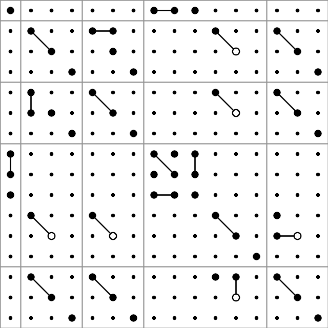
So, this is what we’ll be discussing in this post – preparation of such graphs. We’ll be using the PHP module Imagick for ImageMagick functions and objects. On Ubuntu, you can install the package from the command line as:

sudo apt-get install php5-imagick

(don’t forget to restart the http server if you’re working via a web interface instead of cli)

Before going further into the graph production, here is a description of producing a random matrix compatible with the given conditions in Octave:

Constructing a sample matrix in Octave

clear;

# Declare the matrix
T=[];

# == >> === non-zero coefficients ===== 0 =====
# I used the shorcuts and scripting of Vim to easily format the like lines..
non_zero_coeff = [];
non_zero_coeff = [non_zero_coeff; 1 1];
non_zero_coeff = [non_zero_coeff; 1 8];
non_zero_coeff = [non_zero_coeff; 1 9];
non_zero_coeff = [non_zero_coeff; 1 10];
non_zero_coeff = [non_zero_coeff; 2 2];
non_zero_coeff = [non_zero_coeff; 2 5];
non_zero_coeff = [non_zero_coeff; 2 11];
non_zero_coeff = [non_zero_coeff; 2 14];
non_zero_coeff = [non_zero_coeff; 3 3];
non_zero_coeff = [non_zero_coeff; 3 6];
non_zero_coeff = [non_zero_coeff; 3 12];
non_zero_coeff = [non_zero_coeff; 3 15];
non_zero_coeff = [non_zero_coeff; 4 4];
non_zero_coeff = [non_zero_coeff; 4 7];
non_zero_coeff = [non_zero_coeff; 3 12];
non_zero_coeff = [non_zero_coeff; 4 16];
non_zero_coeff = [non_zero_coeff; 5 5];
non_zero_coeff = [non_zero_coeff; 5 11];
non_zero_coeff = [non_zero_coeff; 1 9];
non_zero_coeff = [non_zero_coeff; 5 14];
non_zero_coeff = [non_zero_coeff; 6 6];
non_zero_coeff = [non_zero_coeff; 6 12];
non_zero_coeff = [non_zero_coeff; 1 9];
non_zero_coeff = [non_zero_coeff; 6 15];
non_zero_coeff = [non_zero_coeff; 7 7];
non_zero_coeff = [non_zero_coeff; 7 16];
non_zero_coeff = [non_zero_coeff; 8 8];
non_zero_coeff = [non_zero_coeff; 8 9];
non_zero_coeff = [non_zero_coeff; 8 10];
non_zero_coeff = [non_zero_coeff; 6 15];
non_zero_coeff = [non_zero_coeff; 9 9];
non_zero_coeff = [non_zero_coeff; 9 10];
non_zero_coeff = [non_zero_coeff; 10 10];
non_zero_coeff = [non_zero_coeff; 11 11];
non_zero_coeff = [non_zero_coeff; 11 14];
non_zero_coeff = [non_zero_coeff; 12 12];
non_zero_coeff = [non_zero_coeff; 12 14];
non_zero_coeff = [non_zero_coeff; 13 13];
non_zero_coeff = [non_zero_coeff; 14 14];
non_zero_coeff = [non_zero_coeff; 15 15];
non_zero_coeff = [non_zero_coeff; 16 16];

# Assign random values to the non-zero coefficients:
for i=1:rows(non_zero_coeff)
T(non_zero_coeff(i,1),non_zero_coeff(i,2)) = rand;
endfor
# == << === non-zero coefficients ===== 1 ===== 

# == >> === Relations ===== 0 =====
T(1,9)=T(1,8);
T(3,3)=T(2,2);
T(2,6)=T(2,5);
T(3,12)=-T(2,11);
T(3,15)=T(2,14);
T(6,6)=T(5,5);
T(6,12)=-T(5,11);
T(6,15)=T(5,14);
T(9,9)=T(8,8);
T(9,10)=T(8,10);
T(12,12)=T(11,11);
T(12,15)=-T(12,14);
T(15,15)=T(14,14);
# == << === Relations ===== 1 ===== 

# == >> === Symmetry ===== 0 =====
for i=1:rows(T)
for j=i:columns(T)
T(j,i) = T(i,j);
endfor
endfor
# == << === Symmetry ===== 1 =====

# Export the matrix to a file:
save("input.data.txt","T");

Finding out the relations between the coefficients

Doing a double loop over i=1:rows and j=i:cols, for each of the coefficients in and above the diagonal, taking one as reference (checking if abs(T(i,j))>0 and recording to an array, say “non-zero-coeff-array” if so) and then comparing it with the rest of the elements (that comes after it) with another double loop i2=i:rows and j2=j:cols. If T(i2,j2) is equal to +-T(i,j), we also note this (three values for each i2,j2 equivalency identification: i2,j2 and +/-1) in another array (say “equal-array”).

For example, according to our case the (9,9) element of the non-zero-coeff-array would be TRUE and the same element of the equal-array would be a sub-array holding the values (8,8,1).

Painting on a canvas

Once you have access to the ImageMagick library through Imagick, we can start “painting” a canvas by first defining the canvas (width, height and background color):

# Declare the object (/holder)
$image = new Imagick();

# Define the canvas (size 640x640 pixels with white background)
$image->newImage( 640, 640, new ImagickPixel( 'white' ) );

Let’s put a circle (filled, black) in the center with a radius of 30 pixels:

# Define the circle:
$circle = new ImagickDraw();
$circle->setFillColor("#000000");
$circle->circle(320,320,350,320);

# Add (/register) it to the canvas:
$image->drawImage($circle);

As for the production of the image file, we need to designate it as a PNG image and then export it to a file:
<code># Designate the image type as PNG:
$image->setImageFormat( "png" );

# Export (/write) it to a file "out.png":
$fp = fopen("out.png","w");
fwrite($fp,$image);
fclose($fp);

This is what you -should- get:

not bad for beginning, right? 😉

The circle function has 4 parameters: the (x,y) coordinates of the center and the coordinates of a point that is on the edge of the circle. Let’s draw another circle, this time an unfilled one below this filled one:

# Declare the object (/holder) 
$image = new Imagick();

 # Define the canvas (size 640x640 pixels with white background)
 $image --->newImage( 640, 640, new ImagickPixel( 'white' ) );

# Define the 1st, filled circle:
$circle = new ImagickDraw();
$circle->setFillColor("#000000");
$circle->circle(320,320,350,320);

# Add (/register) it to the canvas:
$image->drawImage($circle);

# Define the 2nd, unfilled circle:
$circle = new ImagickDraw();
$circle->setStrokeColor("#000000");
$circle->setStrokeWidth(2);
$circle->setFillColor("none");
$circle->circle(320,350,350,350);

# Add (/register) it to the canvas:
$image->drawImage($circle);

# Designate the image type as PNG:
$image->setImageFormat( "png" );

# Export (/write) it to a file "out.png":
$fp = fopen("out.png","w");
fwrite($fp,$image);
fclose($fp);

The “stroke” methods are responsible for the perimeter and the fillcolor setting to “none” ensures that we have an otherwise invisible circle.

So far, so good.. Let’s add a line that passes between the circles from (120,50) to (520,50):

# Define the line:
$line = new ImagickDraw();
$line->setStrokeColor("#000000");
$line->setStrokeWidth(2);
$line->line(120,350,520,350);
$image->drawImage($line);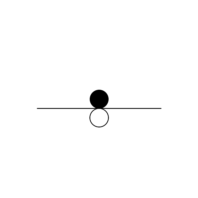

Mapping the rows and cols to x and y

Suppose that we have a 16×16 matrix to be mapped onto a 640×640 canvas. We could map (i=0,j=0) to (x=0,y=0) and (i=16,j=16) to (x=640,y=640) but it wouldn’t be right:

doesn’t look right, right? And here’s the code that produced it:

# Declare the object (/holder)
$image = new Imagick(); 

# Define the canvas (size 640x640 pixels with white background) 
$image--->newImage( 640, 640, new ImagickPixel( 'white' ) );

# Define the 1st, filled circle:
$dxy = 640 / 16;
for($i=1;$i<=16;$i++)
{
for($j=1;$j<=16;$j++)
     {
         $circle = new ImagickDraw();
         $circle->setFillColor("#000000");
         $circle->circle($dxy*($j-1),$dxy*($i-1),$dxy*($j-1)+$dxy/6,$dxy*($i-1));

         # Add (/register) it to the canvas:
         $image->drawImage($circle);
     }
}

# Designate the image type as PNG:
$image->setImageFormat( "png" );

# Export (/write) it to a file "out.png":
$fp = fopen("out.png","w");
fwrite($fp,$image);
fclose($fp);

What we need to do is to shift it half of the periodicity in the x & y directions:

That’s more like it — this shift was introduced to the code by changing the coordinate parameters of the circle(s):
$circle->circle($dxy*($j-1/2),$dxy*($i-1/2),$dxy*($j-1/2)+$dxy/6,$dxy*($i-1/2));

So, depending on the value (zero/non-zero) of an element of our tensor, we can put it as a big circle (r=$dxy/6) or a small one (r=$dxy/12). In addition, if it’s negative, we can have it drawn as an unfilled one (

$circle->setStrokeColor("#000000");
$circle->setStrokeWidth(2);
$circle->setFillColor("none");

). We’re almost ready aside from the connecting the related entries!

Connecting the dots

Suppose that we’d like to connect the circles corresponding to the (i1,j1) and the (i2,j2) elements of the tensor. On the canvas, their centers will be given as ($dxy*($j1-1/2),$dxy*($i1-1/2)) and ($dxy*($j2-1/2),$dxy*($i2-1/2)) where $dxy is the conversion unit of 1 step in the row-col matrix to that of the canvas (for simplicity I assumed a square canvas which is not necessary — then we’d have a $dx=$width/$num_cols and a $dy=$height/$num_rows. Also note that the rows are associated with the height ($i <-> vertical) and the columns are with the width ($j <-> horizontal) (that’s why $j’s come before $i’s in the center equations).

So, let’s join (11,5) to (9,3): in a 640×640 canvas, (11,5) is centered at ((640/16)*(5-1/2) = 180, (640/16)*(11-1/2) = 420) and similarly (9,3) is centered at (100,340). Let’s put them on the map and connect their centers with a line:

# Declare the object (/holder)
$image = new Imagick();

# Define the canvas (size 640x640 pixels with white background)
$image->newImage( 640, 640, new ImagickPixel( 'white' ) );

$dxy = 640/16; # 40px
$radius = $dxy/6; #6.6667px

# Define the unfilled (11,5) circle:
$circle = new ImagickDraw();
$circle->setStrokeColor("#000000");
$circle->setStrokeWidth(2);
$circle->setFillColor("none");
$circle->circle(180,420,180+$radius,420);

# Add (/register) it to the canvas:
$image->drawImage($circle);

# Define the unfilled (9,3) circle:
$circle = new ImagickDraw();
$circle->setStrokeColor("#000000");
$circle->setStrokeWidth(2);
$circle->setFillColor("none");
$circle->circle(100,340,100+$radius,340);

# Add (/register) it to the canvas:
$image->drawImage($circle);

# Connect them with a line:
$line = new ImagickDraw();
$line->setStrokeColor("#000000");
$line->setStrokeWidth(2);
$line->line(180,420,100,340);
$image->drawImage($line);

# Designate the image type as PNG:
$image->setImageFormat( "png" );

# Export (/write) it to a file "out.png":
$fp = fopen("out.png","w");
fwrite($fp,$image);
fclose($fp);

Devil is in the details

By now, hopefully you’ve got the idea of how to swing things in your way. In my case, if I spent the 40% of the time doing the things I described, the remaining 60% went in adjusting the line such that it starts on the perimeter of the circle, not from the center of it, i.e.,

and this requires the determination of the angle of the line connecting our nodes. The angle of a line passing through two points (x1,y1) & (x2,y2) is given by: arctan[(y2-y1)/(x2-x1)], where the value is nothing but the A of the y=Ax+B line equation, and we need to translate the beginning and the final points of our line in this direction by an amount of a radius:

# Find the tangent of the line:
$tg = (340-420)/(100-180);
$alpha_radian = atan($tg);
$alpha_deg = $alpha_radian * 180 / M_PI;

# Connect them with a line:
$line = new ImagickDraw();
$line->setStrokeColor("#000000");
$line->setStrokeWidth(2);
$line->line(180-$radius*cos($alpha_radian),420-$radius*sin($alpha_radian),100+  $radius*cos($alpha_radian),340+$radius*sin($alpha_radian));
$image->drawImage($line);

and that’s more or less all about it!

One picture is worth a thousand words

You can have a sneak peak of the working code via here: http://144.122.31.125/cgi-bin/cryst/programs/tensor_graph/

Now that we can include comments in our input files and submit our jobs in a tidied up way, it’s time to automatize the “convergence search” process. For this, we’ll be using the same diamond example of the previous entry.

Suppose that we want to calculate the energies corresponding to various values of the lattice parameter a, ranging from 3.2 to 4, incrementing by 2: 3.2, 3.4, … , 4.0

Incrementation:
In bash, you can define a for loop to handle this:

for (( i = 1; i <= 9; i++ ))
do
  echo $i;
done

1
2
3
4
5
6
7
8
9

But to work with rational numbers, things get a little bit complex:

for (( i = 1; i <= 5; i++ ))
do
    val=$(awk "BEGIN {print 3+$i/5 }")
    echo $val;
done

3.2
3.4
3.6
3.8
4

Alas, it is still not very practical to everytime calculate the necessary values to produce our intended range. This is where the mighty Octave once again comes to the rescue: [A:I:B] in Octave defines a range that starts from A, and continues by incrementing by I until B is reached (or exceeded). So, here is our example in Octave:

octave:1> [3.2:0.2:4]
ans =

   3.2000   3.4000   3.6000   3.8000   4.0000

You can generate temporary input scripts for Octave but better yet, you can also feed simple scripts directly to Octave:

sururi@husniya:~/shared/qe/diamond_tutorial$ echo "[3.2:0.2:4]"|octave -q
ans =

   3.2000   3.4000   3.6000   3.8000   4.0000

The “-q” parameter causes Octave to run in “quiet” mode, so we just feed the range via pipe to Octave and will harvest the output. In general, we’d like to keep the “ans =” and the blank lines out, and then, when there are more than 1 line’s worth of output, Octave puts the “Column” information as in:

octave:4> [3:0.1:4]
ans =

 Columns 1 through 9:

   3.0000   3.1000   3.2000   3.3000   3.4000   3.5000   3.6000   3.7000   3.8000

 Columns 10 and 11:

   3.9000   4.0000

all these nuisances can go away via a simple “grep -v” (with the ‘v’ parameter inverting the filter criteria):

sururi@vala:/tmp$ echo "[3.2:0.1:4]"|octave -q|sed -n "2,1000p"| grep -v "Column"

   3.2000   3.3000   3.4000   3.5000   3.6000   3.7000   3.8000   3.9000

   4.0000

sururi@vala:/tmp$ echo "[3.2:0.1:4]"|octave -q|sed -n "2,1000p"| grep -v "Column"|grep -v -e "^$"
   3.2000   3.3000   3.4000   3.5000   3.6000   3.7000   3.8000   3.9000
   4.0000

Replacement:
Now that we have the variable’s changing values, how are we gonna implement it to the input script? By search and replace. Suppose, we have a template in which the variable’s value is specified by “#REPLACE#”, all we need to do is to “sed” the file:

cat diamond.scf.in | sed "s:#REPLACE#:$a:g">tmp_$a.in

where “$a” is the current value in the iteration.

Parsing the Energy:
We submit this job via mpirun (in our case via mpi-pw.x of the previous post) and parse the output for the final energy:

grep -e ! tmp_$a.out|tail -n1|awk '{print $(NF-1)}'

For each iteration we thus obtain the energy for our $a value, so we put them together in two columns into a data file I’d like to call “E_vs_$a.txt”.

The Script:
Putting all these together, here is the script in its full glory:

#!/bin/bash

# Takes in the template Quantum Espresso input file, runs it iteratively
# changing the #REPLACE# parameters iteratively with the range elements,
# grepping the energy and putting it along with the current value of the
# #REPLACE# parameter.
#
# Emre S. Tasci, 03/2012

# Example: Suppose that the file "diamond.scf.in" contains the following line:
#   A = #REPLACE#
# Calling "qe-opti.sh diamond.scf.in a 3.2 0.2 4.2" would cause that line to be modified as
#   A = 3.2
# and submitted, followed by
#   A = 3.4, 3.6, .., 4.2 in the sequential runs.
#
# at the end, having constructed the E_vs_a.txt file.

if [ $# -ne 5 ]
then
    echo "Usage: qe-opti.sh infile_template.in variable_name initial_value increment     final_value"
    echo "Example: qe-opti.sh diamond.scf.in a 3.2 0.2 4.2"
    echo -e "\nNeeds octave to be accessible via \"octave\" command for the range to     work"
    echo -e "\nEmre S. Tasci, 03/2012"
    exit
fi

logext=".txt"
logfilename=E_vs_$2$logext
rm -f $logfilename

range=$(echo "[$3:$4:$5]"|octave -q|sed -n "2,1000p"|grep -vr "^$"|grep -v "Column")
for a in $range
do
    # echo $a
    cat $1|sed "s:#REPLACE#:$a:g">tmp_$a.in
    /home/sururi/bin/mpi-pw.x 4 tmp_$a.in
energ=$(grep -e ! tmp_$a.out|tail -n1|awk '{print $(NF-1)}')
    # echo $energ
    echo -e $a "    " $energ >> $logfilename
    echo -e $a "    " $energ
done

echo "Results stored in: "$logfilename

Action:
Modify the sample input from the previous post so that it’s lattice parameter A is designated as something like “A = #REPLACE#”, as in:

sururi@bebop:~/shared/qe/diamond_tutorial$ grep "REPLACE" -B2 -A2 diamond.scf.in
    # a,b,c in Angstrom =======
    #A = 3.56712
    A = #REPLACE#
    B = 2.49
    C = 2.49

Then call the qe-opti.sh script with the related parameters:

sururi@bebop:~/shared/qe/diamond_tutorial$ qe-opti.sh diamond.scf.in a 3.2 0.2 4.2
Running: mpirun -n 4 /usr/share/espresso-4.3.2/bin/pw.x < tmp_3.2000.in > tmp_3.2000.out

Start : Tue Mar 13 23:21:07 CET 2012
Finish: Tue Mar 13 23:21:08 CET 2012
Elapsed time:0:00:01

3.2000      -22.55859979
Running: mpirun -n 4 /usr/share/espresso-4.3.2/bin/pw.x < tmp_3.4000.in > tmp_3.4000.out

Start : Tue Mar 13 23:21:08 CET 2012
Finish: Tue Mar 13 23:21:09 CET 2012
Elapsed time:0:00:01

3.4000      -22.67717405
Running: mpirun -n 4 /usr/share/espresso-4.3.2/bin/pw.x < tmp_3.6000.in > tmp_3.6000.out

Start : Tue Mar 13 23:21:09 CET 2012
Finish: Tue Mar 13 23:21:10 CET 2012
Elapsed time:0:00:01

3.6000      -22.69824702
Running: mpirun -n 4 /usr/share/espresso-4.3.2/bin/pw.x < tmp_3.8000.in > tmp_3.8000.out

Start : Tue Mar 13 23:21:10 CET 2012
Finish: Tue Mar 13 23:21:11 CET 2012
Elapsed time:0:00:01

3.8000      -22.65805473
Running: mpirun -n 4 /usr/share/espresso-4.3.2/bin/pw.x < tmp_4.0000.in > tmp_4.0000.out

Start : Tue Mar 13 23:21:11 CET 2012
Finish: Tue Mar 13 23:21:13 CET 2012
Elapsed time:0:00:02

4.0000      -22.57776354
Running: mpirun -n 4 /usr/share/espresso-4.3.2/bin/pw.x < tmp_4.2000.in > tmp_4.2000.out

Start : Tue Mar 13 23:21:13 CET 2012
Finish: Tue Mar 13 23:21:14 CET 2012
Elapsed time:0:00:01

4.2000      -22.47538891
Results stored in: E_vs_a.txt

Where the “E_vs_a.txt” contains the … E vs a values!:

sururi@bebop:~/shared/qe/diamond_tutorial$ cat E_vs_a.txt
3.2000      -22.55859979
3.4000      -22.67717405
3.6000      -22.69824702
3.8000      -22.65805473
4.0000      -22.57776354
4.2000      -22.47538891

You can easily plot it using GNUPlot or whatever you want. In my case, I prefer GNUPlot:

sururi@husniya:~/shared/qe/diamond_tutorial$ plot E_vs_a.txt

giving me:

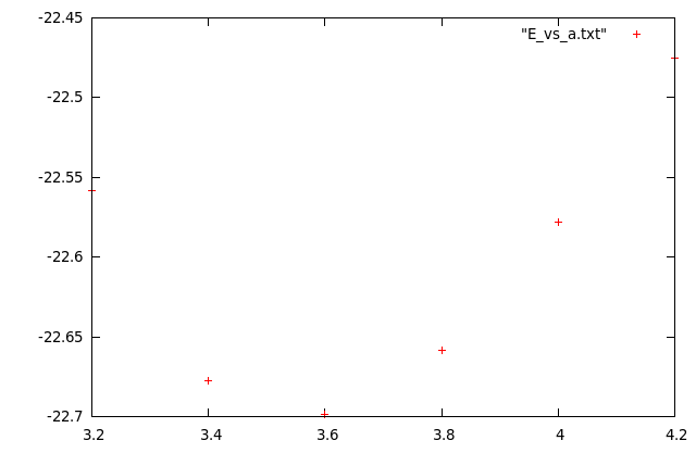
Other than the ‘plot’, I’ve also written another one, fit for data sets just like these where you have a parabol-like data and you’d like to try fitting it and here is what it does (automatically):

sururi@husniya:~/shared/qe/diamond_tutorial$ plotfitparabol.sh E_vs_a.txt
func    f(x)=0.674197*x*x-4.881275*x-13.855234
min, f(min)    3.620066 -22.690502

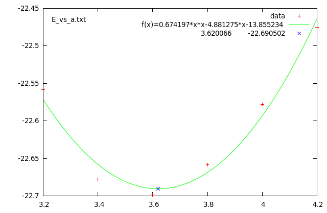
Here are the source codes of the ‘plot’ and ‘plotfitparabol.sh’ scripts. Doei!

sururi@mois:/vala/bin$ cat plot
#!/bin/bash 
gnuplot -persist <<END 
set term postscript enhanced color
set output "$1.ps"
plot "$1" $2 $3

set term wxt
replot
END
sururi@mois:/vala/bin$ cat plotfitparabol.sh 
#!/bin/bash 

# Usage : plotfitparabol.sh <datafile>

# Reads the data points from the given file
# then uses Octave's "polyfit" function to calculate the coefficients 
# for the quadratic fit and also the minimum (maximum) value.
# Afterwards, prepares a GNUPlot script to display:
#    the data set (scatter)
#    fit function
#    the extremum point's value
#
# Written with Quantum Espresso optimizing procedures in mind.

 
if [ $# -ne 1 ]
then
    echo "Usage: plotfitparabol.sh <datafile>"
    echo "Example: plotfitparabol.sh E_vs_A.txt"
    echo -e "\nNeeds octave to be accessible via \"octave\" command to work"
    echo -e "\nEmre S. Tasci <emre.tasci@ehu.es>, 03/2012"
    exit
fi

octave_script="data=load(\"$1\");m=polyfit(data(:,1),data(:,2),2);min=-m(2)*0.5/m(1);fmin=min*min*m(1)+min*m(2)+m(3);printf(\"f(x)=%f*x*x%+f*x%+f|%f\t%f\",m(1),m(2),m(3),min,fmin)"
oct=$(echo $octave_script|octave -q)
#echo $oct

func=${oct/|*/ }
minfmin=${oct/*|/ }
echo -e "func \t" $func
echo -e "min, f(min) \t" $minfmin

echo '$func
set term postscript enhanced color
set label "$1" at graph 0.03, graph 0.94
set output "$1.ps"
plot "$1" title "data", f(x) title "$func", "<echo '$minfmin'" title "$minfmin"

set term wxt
replot'

gnuplot -persist <<END 
$func
set term postscript enhanced color
set label "$1" at graph 0.03, graph 0.94
set output "$1.ps"
plot "$1" title "data", f(x) title "$func", "<echo '$minfmin'" title "$minfmin"

set term wxt
replot
END

In my previous postdoc position, DFT calculations were governing my research field but with my current position at the Bilbao Crystallographic Server, we are more on the theoretical side of things then calculations. Nevertheless, recently, my old ‘flame’ have been kindled and I decided to scrape the rust.

As a change, I selected and installed the Quantum Espresso (QE) package instead of VASP that I was using in the past, main reason QE being open source.

As a newbie to QE and long-gone returner to DFT, I started to practice by mostly ye olde trial/error approach.

The first thing that surprised me the lack of a commenting option in regard to QE input files! (Actually, I’m almost sure that it surely is supported but I have yet to find!). Here’s my sample input file:

&control
    title='Diamond Relaxing',

    # Calculation Type ==========
    calculation='scf'
    #calculation='relax',
    #calculation='vc-relax'
    #calculation='cp'

    # Restart ===================
    restart_mode='from_scratch',
    #restart_mode='restart' 

    # Read/Write units ==========
    #ndr = 51,
    #ndw = 51,

    #nstep = 100,
    #nstep = 1000,
    nstep = 2000,

    # max_seconds = 600 # jobs stops after max_seconds CPU time.

    iprint = 10, # band energies are written every iprint iterations
    #tstress = .TRUE., # calculate stress. It is set to .TRUE. automatically if
                       # calculation='vc-md' or 'vc-relax'
    #tprnfor = .TRUE., # print forces. Set to .TRUE. if calculation='relax','md','vc-md'
    #dt = 5.0d0, # time step for molecular dynamics, in Rydberg atomic units
                 # (1 a.u.=4.8378 * 10^-17 s : beware, the CP code use
                 #  Hartree atomic units, half that much!!!)

    prefix='diamond_rel', # prepended to input/output filenames
    pseudo_dir = '/usr/share/espresso-4.3.2/pseudo/',
    outdir='/home/sururi/shared/tmp/'
    etot_conv_thr = 1.d-6 # convergence threshold on total energy (a.u) for ionic minimization
    forc_conv_thr = 1.d-3 # convergence threshold on forces (a.u) for ionic minimization
 /
 &system
##  ibrav
##    0          "free", see above                 not used
##    1          cubic P (sc)                      not used
##    2          cubic F (fcc)                     not used
##    3          cubic I (bcc)                     not used
##    4          Hexagonal and Trigonal P        celldm(3)=c/a
##    5          Trigonal R, 3fold axis c        celldm(4)=cos(alpha)
##   -5          Trigonal R, 3fold axis <111>    celldm(4)=cos(alpha)
##    6          Tetragonal P (st)               celldm(3)=c/a
##    7          Tetragonal I (bct)              celldm(3)=c/a
##    8          Orthorhombic P                  celldm(2)=b/a,celldm(3)=c/a
##    9          Orthorhombic base-centered(bco) celldm(2)=b/a,celldm(3)=c/a
##   10          Orthorhombic face-centered      celldm(2)=b/a,celldm(3)=c/a
##   11          Orthorhombic body-centered      celldm(2)=b/a,celldm(3)=c/a
##   12          Monoclinic P, unique axis c     celldm(2)=b/a,celldm(3)=c/a,
##                                               celldm(4)=cos(ab)
##  -12          Monoclinic P, unique axis b     celldm(2)=b/a,celldm(3)=c/a,
##                                               celldm(5)=cos(ac)
##   13          Monoclinic base-centered        celldm(2)=b/a,celldm(3)=c/a,
##                                               celldm(4)=cos(ab)
##   14          Triclinic                       celldm(2)= b/a,
##                                               celldm(3)= c/a,
##                                               celldm(4)= cos(bc),
##                                               celldm(5)= cos(ac),
##                                               celldm(6)= cos(ab
    ibrav= 2,

# Cell dimensions ========================
    # a,b,c in Angstrom =======
    A = 3.56712
    B = 2.49
    C = 2.49
    cosAB=0.5
    cosAC=0.5
    cosBC=0.5

    ## OR ##
    ## celldm(1:6) in Bohr =====
    ## 1 Bohr =  0.529177249 A
    ## 1 A = 1.889725989 Bohr
    # celldm(1) = 6.7409 # alat
    # celldm(2) = 4.7054 # b/a
    # celldm(3) = 4.7054 # c/a
    # celldm(4) = 0.5 # cos(ab)
    # celldm(5) = 0.5 # cos(ac)
    # celldm(6) = 0.5 # cos(ab)

   nat=2,
   ntyp= 1,

   ecutwfc = 40, # kinetic energy cutoff (Ry) for wavefunctions
   # ecutrho = 160 # kinetic energy cutoff (Ry) for charge density and potential.
                   # For norm-conserving pseudopotential you should stick to the
                   # default value
   # nbnd = 6 # number of electronic states (bands) to be calculated.
              # Default:
              # for an insulator, nbnd = number of valence bands (nbnd = # of electrons /2);
              # for a metal, 20% more (minimum 4 more)
 /
 &electrons
   emass = 400.d0
   emass_cutoff = 2.5d0

   #electron_dynamics = 'sd' # CP specific
   #electron_dynamics = 'bfgs' # CP specific

  conv_thr = 1D-6 # Convergence threshold for selfconsistency

 /
 &ions
    #ion_dynamics = 'none'
    #ion_dynamics = 'bfgs'
    #ion_dynamics = 'sd'

    # === damping === 0 ==
    # ion_dynamics = 'damp'
    # ion_damping = 0.2
    # ion_velocities = 'zero' # CP specific -- initial ionic velocities
    # === damping === 1 ==

    #ion_nstepe = 10 # CP specific -- number of electronic steps per ionic step. (Def: 1)
 /
 &cell
    cell_dynamics = 'none',
    #cell_dynamics = 'bfgs', # ion_dynamics must be 'bfgs' too
    #cell_dofree = 'xyz'
    #cell_factor = 3
    press = 0.0d,
    # press_conv_thr = 0.05 # Convergence threshold on the pressure for variable cell relaxation
 /
ATOMIC_SPECIES
 C  12.0107 C.pz-vbc.UPF
ATOMIC_POSITIONS
 C 0.0 0.0 0.0
 C 0.25 0.25 0.25
K_POINTS automatic
   4 4 4 1 1 1

so, it’s not the tidiest parameter file around but nevertheless, I’ve included some explanations and it’s easily customizable by simple commenting out, right?…

And then the problem of (yet undiscovered) comments in the QE input files hits us. But with bash, it’s pretty easy. So, if you save the above contents to a file called, say, “diamond.scf.in” and filter it via grep and sed, you’re done:

sururi@husniya:~/shared/qe/diamond_tutorial$ cat diamond.scf.in | grep -v -E "^[\t ]*#" | sed "s:\([^#]*\)#.*:\1:"
&control
    title='Diamond Relaxing',

    calculation='scf'

    restart_mode='from_scratch',

    nstep = 2000,

    iprint = 10, 

    prefix='diamond_rel',
    pseudo_dir = '/usr/share/espresso-4.3.2/pseudo/',
    outdir='/home/sururi/shared/tmp/'
    etot_conv_thr = 1.d-6
    forc_conv_thr = 1.d-3
 /
 &system
    ibrav= 2,

    A = 3.56712
    B = 2.49
    C = 2.49
    cosAB=0.5
    cosAC=0.5
    cosBC=0.5

   nat=2,
   ntyp= 1,

   ecutwfc = 40,
 /
 &electrons
   emass = 400.d0
   emass_cutoff = 2.5d0

  conv_thr = 1D-6 

 /
 &ions

 /
 &cell
    cell_dynamics = 'none',
    press = 0.0d,
 /
ATOMIC_SPECIES
 C  12.0107 C.pz-vbc.UPF
ATOMIC_POSITIONS
 C 0.0 0.0 0.0
 C 0.25 0.25 0.25
K_POINTS automatic
   4 4 4 1 1 1

I’ve installed the QE to take advantage of the cluster nodes via MPI, so I submit my jobs via:

mpirun -n #_of_processes /usr/share/espresso-4.3.2/bin/pw.x < input_file > output_file

which I guess is more or less similar to what you are doing to run your jobs.

So, combining this “comment filtering” and job submission, I’ve written the following bash script (“mpi-pw.x“) to automatize (and keep log of) the job:

sururi@cowboy:~$ cat /home/sururi/bin/mpi-pw.x 
#!/bin/bash

# Script to submit Quantum Espresso jobs via mpi
# EST, Fri Mar  9 17:02:10 CET 2012

function timer()
{
    if [[ $# -eq 0 ]]; then
        echo $(date '+%s')
    else
        local  stime=$1
        etime=$(date '+%s')

        if [[ -z "$stime" ]]; then stime=$etime; fi

        dt=$((etime - stime))
        ds=$((dt % 60))
        dm=$(((dt / 60) % 60))
        dh=$((dt / 3600))
        printf '%d:%02d:%02d' $dh $dm $ds
    fi
}

if [ $# -ne 2 ]
then
    echo "Usage: mpi-pw.x num_of_processes infile.in"
    exit
fi

job=$2
job_wo_ext=${job%.*}

outext=".out"
logext=".log"
echo -e "Running: mpirun -n $1 /usr/share/espresso-4.3.2/bin/pw.x < $2 > $job_wo_ext$outext\n"
echo -e "Running: mpirun -n $1 /usr/share/espresso-4.3.2/bin/pw.x < $2 > $job_wo_ext$outext\n">$job_wo_ext$logext
echo "Start : "$(date)
echo "Start : "$(date)>>$job_wo_ext$logext

# Take out the comments from the input file
#grep -v -E "^[\t ]*#" $2 > in_wo_comments.in.tmp
grep -v -E "^[\t ]*#" $2 | sed "s:\([^#]*\)#.*:\1:" > in_wo_comments.in.tmp

t=$(timer)
mpirun -n $1 /usr/share/espresso-4.3.2/bin/pw.x < in_wo_comments.in.tmp > $job_wo_ext$outext
echo "Finish: "$(date)
echo "Finish: "$(date)>>$job_wo_ext$logext
printf 'Elapsed time:%s\n\n' $(timer $t)
printf 'Elapsed time:%s\n\n' $(timer $t) >>$job_wo_ext$logext

rm -f in_wo_comments.in.tmp

(I’ve picked the “timer” function from Mitch Frazier’s entry in LinuxJournal)

What it does is, really simple: it strips out the extension of the input file ($2 – the second argument in calling); filters out the comments, constructing the temporary input file “in_wo_comments.in.tmp”; starts the timer; submits the job using the number of processes passed in the calling ($1 – first argument) and directs the output to a file whose name is the extension stripped input filename + “.out”; when the job is (this way or that) done, stops the timer and calculates the elapsed time via the ‘timer’ function. During all this time, it prints these information both on screen and to a file called extension stripped input filename + “.log”.

I have a very similar another script called “mpi-cp.x” that I’ve forked for Carr-Parinelli jobs (just search & replace all the occurrences of “mpi-pw.x” with “mpi-cp.x” and you’re done 8).

And here is the script in action:

sururi@cowboy:~/shared/qe/diamond_tutorial$ ll
total 16
drwxr-xr-x 2 sururi sururi 4096 2012-03-13 15:59 ./
drwxr-xr-x 7 sururi sururi 4096 2012-03-13 15:10 ../
-rw-r--r-- 1 sururi sururi 4954 2012-03-13 15:59 diamond.scf.in

sururi@cowboy:~/shared/qe/diamond_tutorial$ mpi-pw.x 4 diamond.scf.in 
Running: mpirun -n 4 /usr/share/espresso-4.3.2/bin/pw.x < diamond.scf.in > diamond.scf.out

Start : Tue Mar 13 16:18:20 CET 2012
Finish: Tue Mar 13 16:18:21 CET 2012
Elapsed time:0:00:01

sururi@cowboy:~/shared/qe/diamond_tutorial$ grep -e ! diamond.scf.out 
!    total energy              =     -22.70063050 Ry

sururi@cowboy:~/shared/qe/diamond_tutorial$ cat diamond.scf.log 
Running: mpirun -n 4 /usr/share/espresso-4.3.2/bin/pw.x < diamond.scf.in > diamond.scf.out

Start : Tue Mar 13 16:18:20 CET 2012
Finish: Tue Mar 13 16:18:21 CET 2012
Elapsed time:0:00:01

Now that we have the mpi-pw.x and mpi-cp.x, our next entry in the series will be the automated search for optimized values.

Suppose that I have a web server which consists of two identical computers behind a splitter that distributes the incoming requests made to a shared ip. Furthermore, the central repository is being kept on a different computer and as a final thing, assume that I sometimes use the computer located in my office, and sometimes the computer at my home as indicated in the following diagram:

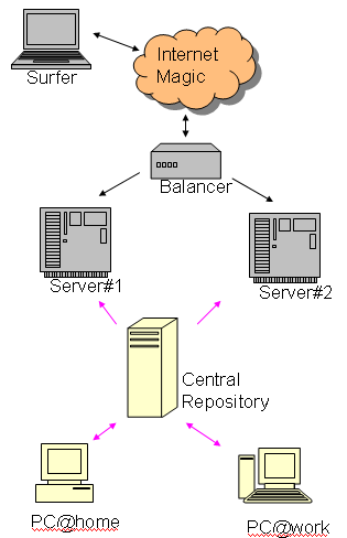
The red arrows indicate the mercurial transfers. You can see that, the changes are only applied to the servers, i.e., nobody codes directly there (no push, only pulls and ups). My two computers can also be thought of two different developers but that part actually isn’t very relevant to this entry’s message. The thing I want to happen is: whenever I push a change into the central repository, I would like to see that it is applied on the servers. In other words I want the following procedures to be automated after the PC@wherever: hg push operation:

1. PC@wherever: hg com
2. PC@wherever: hg push
3. PC@wherever: ssh CentralRepo
4. CentralRepo: hg up
5. CentralRepo: ssh Server#1
6. Server#1: hg pull
7. Server#1: hg up
8. Server#1: ssh Server#2
9. Server#2: hg pull
10. Server#2: hg up

Even though I’ll be using Mercurial in this entry, SVN implementation is pretty much similar. After all, we’ll be using the so-called hooks, i.e. the procedures that takes place upon a triggered event such as push.

Since we will be automating (and I’ll be using SSH for the communication between the nodes), it is essential that the nodes can communicate freely via the help of the ssh-keys (all the relevant information including the usage of “hg-ssh” can be found in a previous entry titled ‘Accessing Mercurial with limited SSH access using key and hg-ssh’).

The trigger event is the incoming data to the central repository, so we edit the .hg/hgrc file of the project on the central repository and type:

[hooks]
incoming = .hg/incominghook.sh > /dev/null

This hook just tells the mercurial to execute the ‘incominghook.sh’ script in the .hg directory (relative to the project’s root dir) whenever there’s an incoming data (i.e., “a push to this -central- repository). So what it should do? It should ‘hg up’ the central repository, for starters. Then, it should ‘ping’ the two servers so that they also pull and update from the -now up-to-date- central repository. This is what the incoming.sh script looks like:

#!/bin/sh
# Go to the project's dir no matter where you are
cd /path/to/the/project/repository/  

# Update it (since this is the central repo, there is no need to 'pull',
#                everybody is pushing to here)
hg up  

# Connect to the servers using the id files specifically generated for this purpose
# so that, upon connection, filtered by the command option
ssh -i ~/.ssh/id_rsa_specific_id_for_the_project__central_repo server1
ssh -i ~/.ssh/id_rsa_specific_id_for_the_project__central_repo server2

Again, if it is not very clear how will the servers get into action by a mere SSH connection, I do urge you to check the aforementioned entry.

The ~/.ssh/authorized_keys file on server1 contains the following related entry corresponding to the supplied id being used in the connection made from central repo:

command="/home/sururi/bin/hgpull_project_x.sh",
no-port-forwarding,no-X11-forwarding,no-agent-forwarding,no-pty
ssh-rsa AAAAB3NzaC1yc2EAAAABIwAAAQEAnq.....==sururi@centralRepo (project X)

So that, when “somebody” connects with the relevant key_id file, the server executes the ‘hgpull_project_x.sh’ (located at /home/sururi/bin/) and returns the output, if any. You can guess that this script actually goes to the project’s location, pulls the changes and then ups it. As is evident from the contents of the ‘hgpull_project_x.sh’ script:

cd /path/to/the/project/on/server1
hg pull --ssh "ssh -i ~/.ssh/id_rsa_specific_id_for_the_project__server1" ssh://sururi@centralrepo//path/to/project
hg up

As you can learn from the strongly referred previous entry, the corresponding line on central repo’s authorized_keys file is something like:

command="hg-ssh /path/to/project/",no-port-forwarding,
no-X11-forwarding,no-agent-forwarding,no-pty ssh-rsa AAAAB...

and we’re done.

Today, I wondered about (actually needed) the possibility to be able to limit (and hence connect afterwards) the access to the repository center of mercurial, using SSH.

To limit an SSH connection, you use ssh-keys: you create a pair of keys, private and public, using the ‘ssh-keygen’ command and then adding the public one to the ~/.ssh/authorized_keys. As an example, consider two computers ‘local’ and ‘remote’ and we want to connect to remote from local without having to enter password every time. So, from the console of local, first I create the key pair:

sururi@local:/tmp/tmp$ ssh-keygen
Generating public/private rsa key pair.
Enter file in which to save the key (/home/sururi/.ssh/id_rsa): ./id_rsa_example
Enter passphrase (empty for no passphrase):
Enter same passphrase again:
Your identification has been saved in ./id_rsa_example.
Your public key has been saved in ./id_rsa_example.pub.
The key fingerprint is:
84:59:8d:8c:43:4a:bc:31:ff:5a:12:23:34:45:56:67 sururi@remote
The key's randomart image is:
+--[ RSA 2048]----+
|   oAE*=A+o      |
|  .o.=..+=..     |
|   .o...         |
|                 |
|        XXX      |
+-----------------+

I didn’t specified any password because I’m intending to have it used automatically (in the hook procedures) and I specified the location of the pair files as the current directory with the names: id_rsa_example  & id_rsa_example.pub

Now, I should append the contents of the ‘id_rsa_example.pub’ file to the ./ssh/authorized_keys at the remote computer. To do this, of course, I should be able to connect it via SSH by normal means. So I execute (from the local computer):

ssh your_username@remote 'cat >> ~/.ssh/authorized_keys' < ./id_rsa_example.pub

And from this moment on -hopefully- you should be able to connect without the remote asking for your password (since we’re not using the default place & filename for the key, i.e. ~/.ssh/id_rsa and ~/.ssh/id_rsa.pub, this newly generated key should be included with the “-i” (identity file) option as in: ssh -i /tmp/tmp/id_rsa_example yourusername:remote)… but, that wasn’t exactly what we wanted. We are thinking of a scenario where you’d like to (semi-)freely distribute the SSH access to the central repository to your developers while making sure that they wouldn’t (couldn’t) do something nasty while they are connected to the remote computer.

We can limit the things an SSH-connected user can do to a single thing via the authorized keys option. Checking this file on the remote computer’s ~/.ssh/authorized_keys file, you should see something like:

ssh-rsa AAAAB3NzaC1yc2EAAAABIwAAAQEAnq5rMLnoab+2F28g/nb58RBENWtX395TuyDFsYkalGaZxrziwDoau/wglkU19DbcAVKgw0p6lMEIuh2iALOppRzxrTgFFhJkL1dxzkugbbPEoSWyfrj9FivzpnxHWgRHQApQeWUBOZhroDTURwfqcyC9SW020CR57jLWfgw+idqwtCu+ZBYmEyHSJcZIH2mWXLrUQ8OalxCFVaLKL50Lpc7V8XJPs+Pg6MPVgfDUqMdjrGkAF7j4viOHTjDWP1h4Ngim70dOeyxWtuqbCbxM4APTShaqET42sj1jHxL2m1dJzXX8s/gEdN0O09hZPhI6rlC+ANWIdJ1vJfODMXWaQ== sururi@local

By adding the “command” option to the beginning of this line would make sure that whenever somebody with the corresponding key connects, that command is run automatically, the results passed back and the connection is terminated afterwards. So, far example. modifying the entry upstairs as:

command="date" ssh-rsa AAAAB3NzaC1yc2EAAAABIwAAAQEAnq5rMLnoab+2F28g/nb58RBENWtX395TuyDFsYkalGaZxrziwDoau/wglkU19DbcAVKgw0p6lMEIuh2iALOppRzxrTgFFhJkL1dxzkugbbPEoSWyfrj9FivzpnxHWgRHQApQeWUBOZhroDTURwfqcyC9SW020CR57jLWfgw+idqwtCu+ZBYmEyHSJcZIH2mWXLrUQ8OalxCFVaLKL50Lpc7V8XJPs+Pg6MPVgfDUqMdjrGkAF7j4viOHTjDWP1h4Ngim70dOeyxWtuqbCbxM4APTShaqET42sj1jHxL2m1dJzXX8s/gEdN0O09hZPhI6rlC+ANWIdJ1vJfODMXWaQ== sururi@local== sururi@vala

would cause the following behaviour from the remote:

sururi@local:~$ ssh -i /tmp/tmp/id_rsa_example sururi@remote
Sun Aug 28 22:05:54 CEST 2011
Connection to remote closed.

I’m a bit tired now writing in full details, so will skip some obvious things from now on. Mercurial has an SSH-wrapper called ‘hg-ssh’ exactly for this purpose, and you can use it by specifying the paths of the repositories as command arguments as in:

command="hg-ssh /path/to/repository" ssh-rsa AAAAB3NzaC1yc2EAAAABIwAAAQEAnq5rMLnoab+2F28g/nb58RBENWtX395TuyDFsYkalGaZxrziwDoau/wglkU19DbcAVKgw0p6lMEIuh2iALOppRzxrTgFFhJkL1dxzkugbbPEoSWyfrj9FivzpnxHWgRHQApQeWUBOZhroDTURwfqcyC9SW020CR57jLWfgw+idqwtCu+ZBYmEyHSJcZIH2mWXLrUQ8OalxCFVaLKL50Lpc7V8XJPs+Pg6MPVgfDUqMdjrGkAF7j4viOHTjDWP1h4Ngim70dOeyxWtuqbCbxM4APTShaqET42sj1jHxL2m1dJzXX8s/gEdN0O09hZPhI6rlC+ANWIdJ1vJfODMXWaQ== sururi@local

(and for more security, I would suggest you include the other options as well, such as:)

command="hg-ssh /path/to/repository",no-port-forwarding,no-X11-forwarding,no-agent-forwarding,no-pty ssh-rsa AAAAB3NzaC1yc2EAAAABIwAAAQEAnq5rMLnoab+2F28g/nb58RBENWtX395TuyDFsYkalGaZxrziwDoau/wglkU19DbcAVKgw0p6lMEIuh2iALOppRzxrTgFFhJkL1dxzkugbbPEoSWyfrj9FivzpnxHWgRHQApQeWUBOZhroDTURwfqcyC9SW020CR57jLWfgw+idqwtCu+ZBYmEyHSJcZIH2mWXLrUQ8OalxCFVaLKL50Lpc7V8XJPs+Pg6MPVgfDUqMdjrGkAF7j4viOHTjDWP1h4Ngim70dOeyxWtuqbCbxM4APTShaqET42sj1jHxL2m1dJzXX8s/gEdN0O09hZPhI6rlC+ANWIdJ1vJfODMXWaQ== sururi@local

and you can pull now on the local computer from the central repository at the remote computer with a command like:

sururi@local:~/project$ hg pull --ssh "ssh -i /tmp/tmp/id_rsa_example" ssh://sururi@remote//path/to/repo
pulling from ssh://sururi@remote//path/to/repo
searching for changes
no changes found