Hex, Bugs and More Physics | Emre S. Tasci

Recently, we needed to schematize the relations between the coefficients of a symmetric tensor matrix such that, beyond the tedious numerical values, the basic relations such as equivalency or (-1) times would be visible to the eye.

Consider the following 16×16 matrix:

   0.06483   0.00000   0.00000   0.00000   0.00000   0.00000   0.00000   0.65809   0.65809   0.60365   0.00000   0.00000   0.00000   0.00000   0.00000   0.00000
   0.00000   0.10993   0.00000   0.00000   0.37862   0.37862   0.00000   0.00000   0.00000   0.00000   0.86568   0.00000   0.00000   0.42424   0.00000   0.00000
   0.00000   0.00000   0.10993   0.00000   0.00000   0.12949   0.00000   0.00000   0.00000   0.00000   0.00000  -0.86568   0.00000   0.00000   0.42424   0.00000
   0.00000   0.00000   0.00000   0.10259   0.00000   0.00000   0.84469   0.00000   0.00000   0.00000   0.00000   0.00000   0.00000   0.00000   0.00000   0.73695
   0.00000   0.37862   0.00000   0.00000   0.01584   0.00000   0.00000   0.00000   0.00000   0.00000   0.84812   0.00000   0.00000   0.87983   0.00000   0.00000
   0.00000   0.37862   0.12949   0.00000   0.00000   0.01584   0.00000   0.00000   0.00000   0.00000   0.00000  -0.84812   0.00000   0.00000   0.87983   0.00000
   0.00000   0.00000   0.00000   0.84469   0.00000   0.00000   0.01168   0.00000   0.00000   0.00000   0.00000   0.00000   0.00000   0.00000   0.00000   0.87050
   0.65809   0.00000   0.00000   0.00000   0.00000   0.00000   0.00000   0.88440   0.28986   0.45572   0.00000   0.00000   0.00000   0.00000   0.00000   0.00000
   0.65809   0.00000   0.00000   0.00000   0.00000   0.00000   0.00000   0.28986   0.88440   0.45572   0.00000   0.00000   0.00000   0.00000   0.00000   0.00000
   0.60365   0.00000   0.00000   0.00000   0.00000   0.00000   0.00000   0.45572   0.45572   0.89801   0.00000   0.00000   0.00000   0.00000   0.00000   0.00000
   0.00000   0.86568   0.00000   0.00000   0.84812   0.00000   0.00000   0.00000   0.00000   0.00000   0.35993   0.00000   0.00000   0.19336   0.00000   0.00000
   0.00000   0.00000  -0.86568   0.00000   0.00000  -0.84812   0.00000   0.00000   0.00000   0.00000   0.00000   0.35993   0.00000   0.62239  -0.62239   0.00000
   0.00000   0.00000   0.00000   0.00000   0.00000   0.00000   0.00000   0.00000   0.00000   0.00000   0.00000   0.00000   1.18908   0.00000   0.00000   0.00000
   0.00000   0.42424   0.00000   0.00000   0.87983   0.00000   0.00000   0.00000   0.00000   0.00000   0.19336   0.62239   0.00000   0.54930   0.00000   0.00000
   0.00000   0.00000   0.42424   0.00000   0.00000   0.87983   0.00000   0.00000   0.00000   0.00000   0.00000  -0.62239   0.00000   0.00000   0.54930   0.00000
   0.00000   0.00000   0.00000   0.73695   0.00000   0.00000   0.87050   0.00000   0.00000   0.00000   0.00000   0.00000   0.00000   0.00000   0.00000   0.55094

if you really want to, you can verify that its coefficients satisfy the following properties:
Non-zero Elements:
(1,1), (1,8), (1,9), (1,10),
(2,2), (2,5), (2,6), (2,11), (2,14),
(3,3), (3,6), (3,12), (3,15),
(4,4), (4,7), (4,16),
(5,5), (5,11), (5,14),
(6,6), (6,12), (6,15),
(7,7), (7,16),
(8,8), (8,9), (8,10),
(9,9), (9,10),
(10,10),
(11,11), (11,14),
(12,12), (12,14), (12,15),
(13,13), (14,14), (15,15),
(16,16)

Equality relations:
(1,9) = (1,8)
(3,3) = (2,2)
(2,6) = (2,5)
(3,12) = -(2,11)
(3,15) = (2,14)
(6,6) = (5,5)
(6,12) = -(5,11)
(6,15) = (5,14)
(9,9) = (8,8)
(9,10) = (8,10)
(12,12) = (11,11)
(12,15) = -(12,14)
(15,15) = (14,14)

These kind of relations are sought upon tensor matrices (at least, in group theory 8), kind of postulating the imposed limits and… (have I said “relations”?). So, the sort-of-important-like thingy is to be able to spot them after evaluating some calculations in the computers.

Have you verified yet? Good! Now let’s take a look at this:

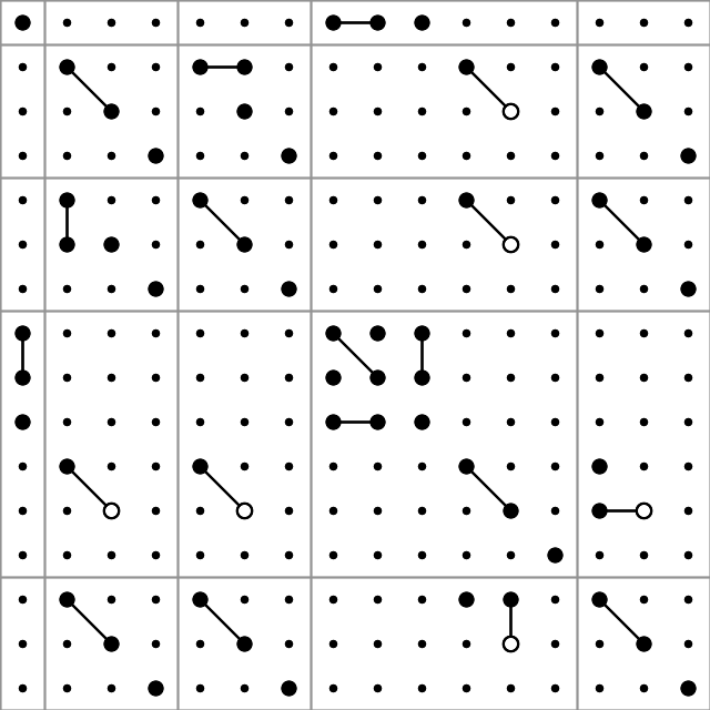
So, this is what we’ll be discussing in this post – preparation of such graphs. We’ll be using the PHP module Imagick for ImageMagick functions and objects. On Ubuntu, you can install the package from the command line as:

sudo apt-get install php5-imagick

(don’t forget to restart the http server if you’re working via a web interface instead of cli)

Before going further into the graph production, here is a description of producing a random matrix compatible with the given conditions in Octave:

Constructing a sample matrix in Octave

clear;

# Declare the matrix
T=[];

# == >> === non-zero coefficients ===== 0 =====
# I used the shorcuts and scripting of Vim to easily format the like lines..
non_zero_coeff = [];
non_zero_coeff = [non_zero_coeff; 1 1];
non_zero_coeff = [non_zero_coeff; 1 8];
non_zero_coeff = [non_zero_coeff; 1 9];
non_zero_coeff = [non_zero_coeff; 1 10];
non_zero_coeff = [non_zero_coeff; 2 2];
non_zero_coeff = [non_zero_coeff; 2 5];
non_zero_coeff = [non_zero_coeff; 2 11];
non_zero_coeff = [non_zero_coeff; 2 14];
non_zero_coeff = [non_zero_coeff; 3 3];
non_zero_coeff = [non_zero_coeff; 3 6];
non_zero_coeff = [non_zero_coeff; 3 12];
non_zero_coeff = [non_zero_coeff; 3 15];
non_zero_coeff = [non_zero_coeff; 4 4];
non_zero_coeff = [non_zero_coeff; 4 7];
non_zero_coeff = [non_zero_coeff; 3 12];
non_zero_coeff = [non_zero_coeff; 4 16];
non_zero_coeff = [non_zero_coeff; 5 5];
non_zero_coeff = [non_zero_coeff; 5 11];
non_zero_coeff = [non_zero_coeff; 1 9];
non_zero_coeff = [non_zero_coeff; 5 14];
non_zero_coeff = [non_zero_coeff; 6 6];
non_zero_coeff = [non_zero_coeff; 6 12];
non_zero_coeff = [non_zero_coeff; 1 9];
non_zero_coeff = [non_zero_coeff; 6 15];
non_zero_coeff = [non_zero_coeff; 7 7];
non_zero_coeff = [non_zero_coeff; 7 16];
non_zero_coeff = [non_zero_coeff; 8 8];
non_zero_coeff = [non_zero_coeff; 8 9];
non_zero_coeff = [non_zero_coeff; 8 10];
non_zero_coeff = [non_zero_coeff; 6 15];
non_zero_coeff = [non_zero_coeff; 9 9];
non_zero_coeff = [non_zero_coeff; 9 10];
non_zero_coeff = [non_zero_coeff; 10 10];
non_zero_coeff = [non_zero_coeff; 11 11];
non_zero_coeff = [non_zero_coeff; 11 14];
non_zero_coeff = [non_zero_coeff; 12 12];
non_zero_coeff = [non_zero_coeff; 12 14];
non_zero_coeff = [non_zero_coeff; 13 13];
non_zero_coeff = [non_zero_coeff; 14 14];
non_zero_coeff = [non_zero_coeff; 15 15];
non_zero_coeff = [non_zero_coeff; 16 16];

# Assign random values to the non-zero coefficients:
for i=1:rows(non_zero_coeff)
T(non_zero_coeff(i,1),non_zero_coeff(i,2)) = rand;
endfor
# == << === non-zero coefficients ===== 1 ===== 

# == >> === Relations ===== 0 =====
T(1,9)=T(1,8);
T(3,3)=T(2,2);
T(2,6)=T(2,5);
T(3,12)=-T(2,11);
T(3,15)=T(2,14);
T(6,6)=T(5,5);
T(6,12)=-T(5,11);
T(6,15)=T(5,14);
T(9,9)=T(8,8);
T(9,10)=T(8,10);
T(12,12)=T(11,11);
T(12,15)=-T(12,14);
T(15,15)=T(14,14);
# == << === Relations ===== 1 ===== 

# == >> === Symmetry ===== 0 =====
for i=1:rows(T)
for j=i:columns(T)
T(j,i) = T(i,j);
endfor
endfor
# == << === Symmetry ===== 1 =====

# Export the matrix to a file:
save("input.data.txt","T");

Finding out the relations between the coefficients

Doing a double loop over i=1:rows and j=i:cols, for each of the coefficients in and above the diagonal, taking one as reference (checking if abs(T(i,j))>0 and recording to an array, say “non-zero-coeff-array” if so) and then comparing it with the rest of the elements (that comes after it) with another double loop i2=i:rows and j2=j:cols. If T(i2,j2) is equal to +-T(i,j), we also note this (three values for each i2,j2 equivalency identification: i2,j2 and +/-1) in another array (say “equal-array”).

For example, according to our case the (9,9) element of the non-zero-coeff-array would be TRUE and the same element of the equal-array would be a sub-array holding the values (8,8,1).

Painting on a canvas

Once you have access to the ImageMagick library through Imagick, we can start “painting” a canvas by first defining the canvas (width, height and background color):

# Declare the object (/holder)
$image = new Imagick();

# Define the canvas (size 640x640 pixels with white background)
$image->newImage( 640, 640, new ImagickPixel( 'white' ) );

Let’s put a circle (filled, black) in the center with a radius of 30 pixels:

# Define the circle:
$circle = new ImagickDraw();
$circle->setFillColor("#000000");
$circle->circle(320,320,350,320);

# Add (/register) it to the canvas:
$image->drawImage($circle);

As for the production of the image file, we need to designate it as a PNG image and then export it to a file:
<code># Designate the image type as PNG:
$image->setImageFormat( "png" );

# Export (/write) it to a file "out.png":
$fp = fopen("out.png","w");
fwrite($fp,$image);
fclose($fp);

This is what you -should- get:

not bad for beginning, right? 😉

The circle function has 4 parameters: the (x,y) coordinates of the center and the coordinates of a point that is on the edge of the circle. Let’s draw another circle, this time an unfilled one below this filled one:

# Declare the object (/holder) 
$image = new Imagick();

 # Define the canvas (size 640x640 pixels with white background)
 $image --->newImage( 640, 640, new ImagickPixel( 'white' ) );

# Define the 1st, filled circle:
$circle = new ImagickDraw();
$circle->setFillColor("#000000");
$circle->circle(320,320,350,320);

# Add (/register) it to the canvas:
$image->drawImage($circle);

# Define the 2nd, unfilled circle:
$circle = new ImagickDraw();
$circle->setStrokeColor("#000000");
$circle->setStrokeWidth(2);
$circle->setFillColor("none");
$circle->circle(320,350,350,350);

# Add (/register) it to the canvas:
$image->drawImage($circle);

# Designate the image type as PNG:
$image->setImageFormat( "png" );

# Export (/write) it to a file "out.png":
$fp = fopen("out.png","w");
fwrite($fp,$image);
fclose($fp);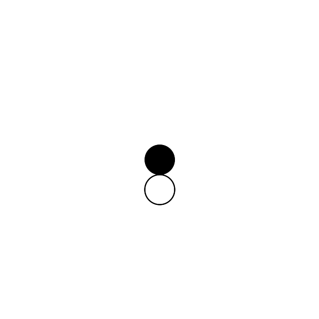

The “stroke” methods are responsible for the perimeter and the fillcolor setting to “none” ensures that we have an otherwise invisible circle.

So far, so good.. Let’s add a line that passes between the circles from (120,50) to (520,50):

# Define the line:
$line = new ImagickDraw();
$line->setStrokeColor("#000000");
$line->setStrokeWidth(2);
$line->line(120,350,520,350);
$image->drawImage($line);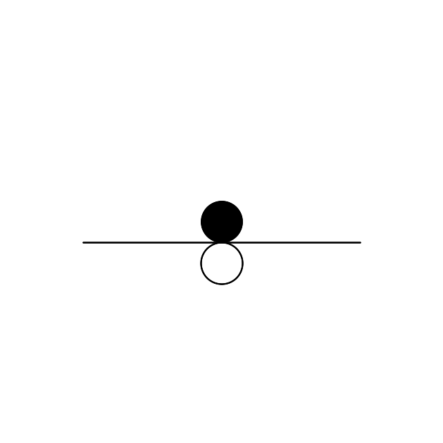

Mapping the rows and cols to x and y

Suppose that we have a 16×16 matrix to be mapped onto a 640×640 canvas. We could map (i=0,j=0) to (x=0,y=0) and (i=16,j=16) to (x=640,y=640) but it wouldn’t be right:

doesn’t look right, right? And here’s the code that produced it:

# Declare the object (/holder)
$image = new Imagick(); 

# Define the canvas (size 640x640 pixels with white background) 
$image--->newImage( 640, 640, new ImagickPixel( 'white' ) );

# Define the 1st, filled circle:
$dxy = 640 / 16;
for($i=1;$i<=16;$i++)
{
for($j=1;$j<=16;$j++)
     {
         $circle = new ImagickDraw();
         $circle->setFillColor("#000000");
         $circle->circle($dxy*($j-1),$dxy*($i-1),$dxy*($j-1)+$dxy/6,$dxy*($i-1));

         # Add (/register) it to the canvas:
         $image->drawImage($circle);
     }
}

# Designate the image type as PNG:
$image->setImageFormat( "png" );

# Export (/write) it to a file "out.png":
$fp = fopen("out.png","w");
fwrite($fp,$image);
fclose($fp);

What we need to do is to shift it half of the periodicity in the x & y directions:

That’s more like it — this shift was introduced to the code by changing the coordinate parameters of the circle(s):
$circle->circle($dxy*($j-1/2),$dxy*($i-1/2),$dxy*($j-1/2)+$dxy/6,$dxy*($i-1/2));

So, depending on the value (zero/non-zero) of an element of our tensor, we can put it as a big circle (r=$dxy/6) or a small one (r=$dxy/12). In addition, if it’s negative, we can have it drawn as an unfilled one (

$circle->setStrokeColor("#000000");
$circle->setStrokeWidth(2);
$circle->setFillColor("none");

). We’re almost ready aside from the connecting the related entries!

Connecting the dots

Suppose that we’d like to connect the circles corresponding to the (i1,j1) and the (i2,j2) elements of the tensor. On the canvas, their centers will be given as ($dxy*($j1-1/2),$dxy*($i1-1/2)) and ($dxy*($j2-1/2),$dxy*($i2-1/2)) where $dxy is the conversion unit of 1 step in the row-col matrix to that of the canvas (for simplicity I assumed a square canvas which is not necessary — then we’d have a $dx=$width/$num_cols and a $dy=$height/$num_rows. Also note that the rows are associated with the height ($i <-> vertical) and the columns are with the width ($j <-> horizontal) (that’s why $j’s come before $i’s in the center equations).

So, let’s join (11,5) to (9,3): in a 640×640 canvas, (11,5) is centered at ((640/16)*(5-1/2) = 180, (640/16)*(11-1/2) = 420) and similarly (9,3) is centered at (100,340). Let’s put them on the map and connect their centers with a line:

# Declare the object (/holder)
$image = new Imagick();

# Define the canvas (size 640x640 pixels with white background)
$image->newImage( 640, 640, new ImagickPixel( 'white' ) );

$dxy = 640/16; # 40px
$radius = $dxy/6; #6.6667px

# Define the unfilled (11,5) circle:
$circle = new ImagickDraw();
$circle->setStrokeColor("#000000");
$circle->setStrokeWidth(2);
$circle->setFillColor("none");
$circle->circle(180,420,180+$radius,420);

# Add (/register) it to the canvas:
$image->drawImage($circle);

# Define the unfilled (9,3) circle:
$circle = new ImagickDraw();
$circle->setStrokeColor("#000000");
$circle->setStrokeWidth(2);
$circle->setFillColor("none");
$circle->circle(100,340,100+$radius,340);

# Add (/register) it to the canvas:
$image->drawImage($circle);

# Connect them with a line:
$line = new ImagickDraw();
$line->setStrokeColor("#000000");
$line->setStrokeWidth(2);
$line->line(180,420,100,340);
$image->drawImage($line);

# Designate the image type as PNG:
$image->setImageFormat( "png" );

# Export (/write) it to a file "out.png":
$fp = fopen("out.png","w");
fwrite($fp,$image);
fclose($fp);

Devil is in the details

By now, hopefully you’ve got the idea of how to swing things in your way. In my case, if I spent the 40% of the time doing the things I described, the remaining 60% went in adjusting the line such that it starts on the perimeter of the circle, not from the center of it, i.e.,

and this requires the determination of the angle of the line connecting our nodes. The angle of a line passing through two points (x1,y1) & (x2,y2) is given by: arctan[(y2-y1)/(x2-x1)], where the value is nothing but the A of the y=Ax+B line equation, and we need to translate the beginning and the final points of our line in this direction by an amount of a radius:

# Find the tangent of the line:
$tg = (340-420)/(100-180);
$alpha_radian = atan($tg);
$alpha_deg = $alpha_radian * 180 / M_PI;

# Connect them with a line:
$line = new ImagickDraw();
$line->setStrokeColor("#000000");
$line->setStrokeWidth(2);
$line->line(180-$radius*cos($alpha_radian),420-$radius*sin($alpha_radian),100+  $radius*cos($alpha_radian),340+$radius*sin($alpha_radian));
$image->drawImage($line);

and that’s more or less all about it!

One picture is worth a thousand words

You can have a sneak peak of the working code via here: http://144.122.31.125/cgi-bin/cryst/programs/tensor_graph/