Hex, Bugs and More Physics | Emre S. Tasci

Now that I’ve started to once again updating this scientific blog of mine, let me also talk about the things that occured since the last entry on October (or even going before that).

Meeting with Dr. Villars
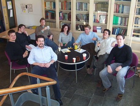
The biggest event that occured to me was meeting with Dr. Pierre Villars, the person behind the Pauling File database which I have benefitted and still benefitting from. When I had registered to the “MITS 2008 – International Symposium on Materials Database”, an event hosted by the NIMS Materials Database, I had no idea that Dr. Villars would also be attending to the event, so it was a real surprise learning afterwards that I’d have a chance to meet him in person.

You can read the sheer happiness from my face on the occasion of meeting Dr. Villars

Dr. Villars is a very kind and a cheerful person, I had a greatest time knowing him and afterwards I had the privilege of visiting him in his home office in the lovely town of Vitznau, Switzerland where I enjoyed the excellent hospitality of the Villars family. Dr. Villars helped me generously in providing the data in my research project for finding transformation toughening materials through datamining which I’m indebted for.

The MITS 2008 – Int’l Symposium on Materials Database
I was frequently using the databases on the NIMS’ website and had the honour to participate in the last year’s event together with my dear supervisor Dr. Marcel Sluiter. On that occasion, I presented two talks – a materials based one, and another about database query&retrieval methods- titled “Inference from Various Material Properties Using Mutual Information and Clustering Methods” and “Proposal of the XML Specification as a Standard for Materials Database Query and Result Retrieval”, respectively.

I have an ever growing interest on the Japanese Culture since I was a youngster and due to this interest, my expectations from this trip to Japan was high enough for me to be afraid of the fact that I may have disappointed since it was next-to-impossible for anything to fulfill the expectations I had built upon. But, amazingly, I was proved false: the experience I had in Japan were far more superior to anything I had anticipated. The hospitality of the organizing commitee was incredible: everything had been taken care of and everyone was as kind as one could be. I had the chance to meet Dr. Villars as I’ve already wrote about above, and also Dr. Xu, Dr. Vanderah, Dr. Dayal and Dr. Sims and had a great time. It was also due to this meeting, I met a dear friend.

Ongoing Projects
During my time here, I still don’t have anything published and that’s the number one issue that’s bothering me. Apart from my research on the transformation toughening materials, I worked for a time on a question regarding to a related phenomenon, namely about the martensitic transformation mechanism on some transition-metal alloy types. We were able to come up with a nice equation and adequate coefficients that caught the calculation results but couldn’t manage to transfer it to -so to say- a nicely put theory and that doomed the research to being an “ad-hoc” approach. I’ll be returning to it at the first chance I get, so currently, it’s been put on ice (and now remembering how, in the heat of the research I was afraid that someone else would come up with the formula and it would be too late for me.. sad, so sad..). One other (side) project was related to approximate a specific amorphous state in regards with some basis structures obtained using datamining. This project was really exciting and fun to work on because I got to use different methods together: first some datamining, then DFT calculations on the obtained structures and finally thermodynamics to extrapolate to higher temperatures. We’re at the stage of revising the draft at the moment (gratefully!).

Life in the Netherlands & at the TUDelft
It has been almost one and a half year since I started my postdoc here in TUDelft. When we first came here, my daughter was still hadn’t started speaking (yet she had been practicing walking) and now she approximately spent the same amount of time in the Netherlands as she had spent in Turkey (and thankfully, she can speak and also running to everywhere! 8).

When I had come here, I was a nano-physicist, experienced in MD simulations and -independently- a coder when the need arouse. Now, I’m more of a materials guy and coding for the purpose.. 8) I enjoy the wide variety of the jobs & disciplines people around me are working on and definitely benefitting from the works of my friends in our group. I couldn’t ask for more, really. (OK, maybe I’d agree if somebody would come up with an idea for less windy and more sunny weather here in Delft. That’s the one thing I couldn’t still get used to. Delft is a marvelous city with bikes and kind people everywhere, canals full of lillies in the spring, historical buildings everywhere, Amsterdam, Den Haag and Rotterdam just a couple of train stations away and if you wish, Antwerpen, Brussels and Brugges (Belgium) is your next-door neighbour but this dark and closed weather can sometimes be a little mood lowering.) TUDelft is really a wonderful place to be with all the resources and connections that makes you feel you can learn anything and meet anyone that is relevant to the work you’re doing without worrying about the cost. And you’re being kept informed about the events taking place about you through the frequent meetings in your group, in your section, in your department, in your field. I’ve learned a lot and I’m really happy I was accepted here.

(And just when you think I was out of photos!.. 8)

So that’s about the things I’ve enjoyed experiencing and living through.. And I promise, I’ll be posting more regularly and frequently from now on..

Yours the chatty.

After migrating this blog to a new server, I had some difficulties in writing up the equations. It was due to the fact that on this server, I wasn’t able to execute the necessary commands to parse the latex code and convert it to PNG format.

Last week, some need arouse for this and I finally coded the necessary way around to be able to convert LaTeX definitions to their PNG counterparts. Before I start to quote the necessary code and explanations, let me tell that, this method only will work if you can successfully manage to produce this conversation at your -local- computer since what the code does is to generate the image on your local computer and then copy it to the server where your blog (/or whatever you have) resides. So, make sure:

• You can convert LaTeX code to PNG on your -own- computer.
• You are running a httpd server so that the code can copy the output PNG file from your local computer

What the code does:
It has 3 seperate processes. Let’s designate them A, B & C.

• Part A is called on the remote server. It presents a form with textbox in it where you can type the LaTeX code. The form’s target is the same file but this time on your local server, so when you submit the data —
• Part B is called on your local server. Using the texvc code, an open source software that also comes packed with mediawiki, it converts the LaTeX code into a PNG image and places it under the relative math/ directory of your local server. After doing this, via the META tag ‘refresh’ it causes the page to refresh itself loading its correspondence in the remote server, hence initiating —
• Part C where the generated image identified by the MD5 hashname is fetched from the local server and copied unto the relative math/ directory on the remote server. The LaTeX code that was used is also passed in the GET method and it is included in the generated code as the title of the image, so if necessary, the equation can be modified in the future.

The code is as follows:

<?PHP if($_GET["com"]||(!$_POST["formula"] && !$_GET["file"])){?>
<body onload="document.postform.formula.focus();">
<form action="http://yourlocalserver.dns.name/tex/index.php" method="post" name=postform id=postform>
<textarea name="formula" cols=40 rows=5 id=formula>
</textarea><br>
<input type="submit" value="Submit" />
<?PHP
}
if($_POST["formula"])
{
    // NL
    $lol = './texvc  ./mathtemp ./math "'.$_POST["formula"].'" iso-8859-1';
    exec($lol,$out);
    $file = substr($out[0],1,32);
    $formula = base64_encode($_POST["formula"]);
    $html = '<HTML>
<HEAD>
<META http-equiv="refresh" content="0;URL=http://remoteserver.dns.name/tex/index.php?formula='.$formula.'&file='.$file.'">
</HEAD>';
    echo $html;
}
else if($_GET["file"])
{
    // COM
    $file = "math/".$_GET["file"].".png";
    if(!copy("yourlocalserver.dns.name/tex/".$file, $file)) exit( "copy failed<br>");
    $formula = base64_decode($_GET["formula"]);
?>
<form action="http://yourlocalserver.dns.name/tex/index.php" method="post">
<textarea name="formula" cols=40 rows=5><?PHP echo $formula; ?>
</textarea><br>
<input type="submit" value="Submit" />
<?
 
    echo "<br><br><img src=\"".$file."\" title=\"".$formula."\"><br>";
    echo "&lt;img src=\"/tex/".$file."\" title=\"".$formula."\"&gt;<br>";
}
?>

1. Create a directory called ‘tex’ on both servers.
2. Create subdir ‘math’ on both servers
3. Create subdir ‘mathtemp’ on the local server
4. Modify the permissions of these subdirs accordingly
5. Place the executable ‘texvc’ in the ‘tex’ directory
6. Place the code quoted above in the ‘tex’ directories of both servers in a file called ‘index.php’

If everything well up to this point, let’s give it a try and you shall have some output similar to this:

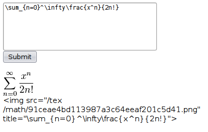
For an input LaTeX code of:
\sum_{n=0}^\infty\frac{x^n}{2n!}

where you can immediately see the resulting image, modify the code if there’s something wrong or copy the IMG tag and put it to your raw HTML input box in your text…

It’s of great importance to have sufficient number of k-points when doing DFT calculations. The most practical (but CPU time costly) way is to check energies for different number of k-points until some kind of "convergence" is reached.

Here are the two scripts I’ve recently written for VASP to check for suitable k-point values.

The first code runs the calculation with increasing k-points (I have a cubic cell, so using same number of k-points for the 3 lattice axes).

Before running this code, make sure that the essential files (KPOINTS POSCAR POTCAR INCAR) are in the directory, also copy your KPOINTS file to a file named "KP" which has KPOINTS mesh defined as 2x2x2:

sururi@husniya Al3Li $ cat KP
Automatic
0
Gamma
2 2 2
0 0 0

The following script will then run the calculations, incrementing the number of K-Points by 1 per each axis. It will store the output (and the 4 input files) in archive files in the format k{%03d}.tar.bz2 where the value in the curly brackets is actually the number of k-points per axis. As you can easily see, it runs from k= 1x1x1 (silly but since this is tutorial) to k=13x13x13.

#!/bin/bash

# A script file to run the system for various k-points in order to find the optimal setting
# Emre S. Tasci, 20/10/2008

for (( i = 1; i <= 13; i++ )) 
do  
    date
    echo $i

    # change the KPOINTS (KP is a copy of the KPOINTS with k=2:
    cat KP|sed s/"2 2 2"/"$i $i $i"/ > KPOINTS

    # run the vasp
    vasp > vasp.out

    # archive the existing files (except the archive files):
    tar -cvjf $(printf "k%02d.tar.bz2" $i) $(ls |grep -v "\(.bz2\)\|\(runrunrun.sh\)\|\(KP$\)\|\(work\)")

    # remove the output files:
    rm $(ls *|grep -v "\(.bz2\)\|\(KPOINTS\)\|\(POSCAR\)\|\(POTCAR\)\|\(INCAR\)\|\(runrunrun.sh\)\|\(KP$\)") -f
    date
    echo "=================================================="
done

After it ends, you should see something like

-rw-r----- 1 sururi users 299K 2008-10-20 10:14 POTCAR
-rw-r--r-- 1 sururi users  283 2008-10-20 10:14 POSCAR
-rw-r--r-- 1 sururi users  604 2008-10-20 10:14 INCAR
-rw-r--r-- 1 sururi users   31 2008-10-20 11:06 KP
-rw-r--r-- 1 sururi users   34 2008-10-20 14:33 KPOINTS
-rw-r--r-- 1 sururi users 195K 2008-10-20 11:08 k01.tar.bz2
-rw-r--r-- 1 sururi users 196K 2008-10-20 11:08 k02.tar.bz2
-rw-r--r-- 1 sururi users 193K 2008-10-20 11:08 k03.tar.bz2
-rw-r--r-- 1 sururi users 195K 2008-10-20 11:08 k04.tar.bz2
-rw-r--r-- 1 sururi users 195K 2008-10-20 11:08 k05.tar.bz2
-rw-r--r-- 1 sururi users 197K 2008-10-20 11:09 k06.tar.bz2
-rw-r--r-- 1 sururi users 197K 2008-10-20 11:09 k07.tar.bz2
-rw-r--r-- 1 sururi users 200K 2008-10-20 11:10 k08.tar.bz2
-rw-r--r-- 1 sururi users 201K 2008-10-20 11:10 k09.tar.bz2
-rw-r--r-- 1 sururi users 205K 2008-10-20 11:11 k10.tar.bz2
-rw-r--r-- 1 sururi users 205K 2008-10-20 11:12 k11.tar.bz2
-rw-r--r-- 1 sururi users 211K 2008-10-20 11:13 k12.tar.bz2
-rw-r--r-- 1 sururi users 211K 2008-10-20 11:14 k13.tar.bz2
-rwxr--r-- 1 sururi users  732 2008-10-20 14:02 runrunrun.sh

Now, it’s time for the second script. Create a new directory (say “work”) and then type the following into a script file (don’t forget to set it as executable (or you can also always “sh ” 😉 ) )

#!/bin/bash
 
# Script name: energy_extract_from_OUTCAR.sh
# Emre S. Tasci, 20/10/2008
 
# Reads the OUTCAR files from the archive files in the parent directory
# Stores the energies in corresponding ENE files.
 
# (Assuming filenames are given like "k05.tar.bz2")
 
k=00
 
for i in ../k*.bz2
do
    kpre=$k
    enepre="0.00000000"
 
    # Extract OUTCAR
    tar -xjf $i OUTCAR
 
    # Parse file counter from filename 
    k=$(echo $(basename $i)|sed "s:k\([0-9]*\).*:\1:")
 
    # write the energies calculated in this run 
    cat OUTCAR | grep "energy without"|awk '{print $8}' > $(printf "%s_ENE" $k)
 
    #calculate the energy difference between this and the last run
    if [ -e "$(printf "%s_ENE" $kpre)" ] 
    then
        enepre=$(tail -n1 $(printf "%s_ENE" $kpre));
    fi
 
    enethis=$(tail -n1 $(printf "%s_ENE" $k));
 
    # Using : awk '{ print ($1 >= 0) ? $1 : 0 - $1}' : for absolute value
 
    echo -e $(printf "%s_ENE" $kpre) " :\t" $enepre "\t" $(printf "%s_ENE" $k) ":\t" $enethis "\t" $(echo $(awk "BEGIN { print $enepre - $enethis}") | awk '{ print ($1 >= 0) ? $1 : 0 - $1}')
 
    rm -f OUTCAR
done;

when runned, this script will produce an output similar to the following:

sururi@husniya work $ ./energy_extract_from_OUTCAR.sh
00_ENE  :        0.00000000      01_ENE :        -6.63108952     6.63109
01_ENE  :        -6.63108952     02_ENE :        -11.59096452    4.95988
02_ENE  :        -11.59096452    03_ENE :        -12.96519853    1.37423
03_ENE  :        -12.96519853    04_ENE :        -13.20466179    0.239463
04_ENE  :        -13.20466179    05_ENE :        -13.26411934    0.0594576
05_ENE  :        -13.26411934    06_ENE :        -13.26528991    0.00117057
06_ENE  :        -13.26528991    07_ENE :        -13.40540825    0.140118
07_ENE  :        -13.40540825    08_ENE :        -13.35505746    0.0503508
08_ENE  :        -13.35505746    09_ENE :        -13.38130280    0.0262453
09_ENE  :        -13.38130280    10_ENE :        -13.36356457    0.0177382
10_ENE  :        -13.36356457    11_ENE :        -13.37065368    0.00708911
11_ENE  :        -13.37065368    12_ENE :        -13.37249683    0.00184315
12_ENE  :        -13.37249683    13_ENE :        -13.38342842    0.0109316

Which shows the final energies of the sequential runs as well as the difference of them. You can easily plot the energies in the gnuplot via as an example “plot “12_ENE”“. You can also plot the evolution of the energy difference with help from awk. To do this, make sure you first pipe the output of the script to a file (say “energies.txt”):

./energy_extract_from_OUTCAR.sh > energies.txt

And then, obtaining the last column via awk

cat energies.txt |awk '{print $7}' > enediff.txt

Now you can also easily plot the difference file.

Hope this scripts will be of any help.

Still saddened by the loss of Randy Pausch whom I knew about from his famous "Last Lecture", while working on the Miedema’s Model, I came across this article by him:

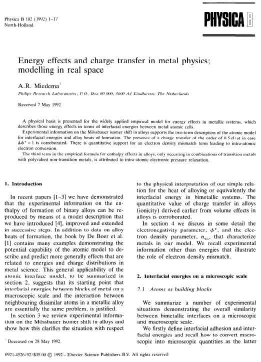
Dr. Villars had already mentioned Miedema’s passing at a young age but still it was really tragic to find such a sad detail on a scientific article.

I checked the web for a Miedema biography but couldn’t find any. The only information I could find was from H. Bakker’s book which I’m quoting the preface below:

PREFACE

   Andries Miedema started developing his rather unconventional model in the sixties as a professor at the University of Amsterdam and continued this work from 1971 at Philips Research Laboratories. At first he encountered scepticism in these environments, where scientists were expecting all solutions from quantum- mechanics. Of course, Miedema did not deny that eventually quantum mechanics could produce (almost) exact solutions of problems in solid-state physics and materials science, but the all-day reality he experienced was, – and still is -, that most practical problems that are encountered by researchers are too complex to allow a solution by application of the Schr6dinger equation. Besides, he believed in simplicity of nature in that sense that elements could be characterised by only a few fundamental quantities, whereby it should be possible to describe alloying behaviour. On the basis of a comparison of his estimates of the heat of formation of intermetallic compounds with ample experimental data, he was gradually able to overcome the scepticism of his colleagues and succeeded in convincing the scientific world that his model made sense. This recognition became distinct by the award of the Hewlett Packard prize in 1980 and the Hume-Rothery decoration in 1981. At that time, Miedema himself and many others were successfully using and extending the model to various questions, of course realising that the numbers obtained by the model have the character of estimates, but estimates that could not be obtained in a different fast way. It opened new perspectives in materials science. Maybe the power of the model is best illustrated by a discussion, the present author had with Jim Davenport at Brookhaven National Laboratory in 1987. Dr Davenport showed him a result that was obtained by a one-month run on a Gray 1 supercomputer. This numerical result turned out to be only a few kilo Joules different from the outcome by Miedema’s model, obtained within a few minutes by use of a pocket calculator. Andries Miedema passed away in 1992 at a much too young age of 59 years. His death came as a bad shock not only for the scientific community in The Netherlands, but for scientists all over the world. However, for his family, friends and all the people, who knew him well, it is at least some consolation that he lives on by his model, which is being used widely and which is now part of many student programmes in physics, chemistry and materials science.

   It is the aim of the present review to make the reader familiar with the application of the model, rather than to go in-depth into the details of the underlying concepts. After studying the text, the reader should be able, with the aid of a number of tables from Miedema’s papers and his book, given in the appendix, to make estimates of desired quantities and maybe even to extend the model to problems that, so far, were not handled by others. Beside, the reader should be aware of the fact that not all applications could be given in this review. For obvious reasons only part of all existing applications are reported and the reader will find further results of using the model in Miedema’s and co-worker’s papers, book and in literature.

   Dr Hans Bakker is an associate professor at the Van der Waals-Zeeman Institute of the University of Amsterdam. In 1970 Andries Miedema was the second supervisor of his thesis on tracer diffusion. He inspired him to subsequent work on diffusion and defects in VIII-IIIA compounds at a time, when, – as Bakker’s talk was recently introduced at a conference -, these materials were not yet relevant’ as they are now. Was it again a foreseeing view of Andries Miedema? Was it not Miedema’s standpoint that intermetallic compounds would become important in the future?

   Rather sceptic about the model as Bakker was at first like his colleagues, his scepticism passed into enthusiasm, when he began using the model with success in many research problems. In 1984 Bakker’s group started as one of the first in the world ball milling experiments. Surprisingly this seemingly crude technique turned out to be able to induce well-defined, non-equilibrium states and transformations in solids. Miedema’s model appeared again to be very helpful in understanding and predicting those phenomena.

Hans Bakker
Mauro Magini

Preface from Enthalpies in Alloys : Miedema’s Semi-Emprical Model
H. Bakker
Trans Tech Publications 1998 USA
ISSN 1422-3597

Yes, it’s been 25 years since A.K. Niessen, A.R. Miedema et al.’s "Model Predictions for the Enthalpy of Formation of Transition Metal Alloys II" titled article (CALPHAD 7(1) 51-70 1983) was published. It can be thought as a sequel to Miedema et al.’s 1979 (Calphad 1 341-359 1979) and 1980 dated (Physica 100 1-28 1980) papers with some update on the data as well as a computer code to calculate the enthalpies of formation written in ALGOL.

I have been currently working on these papers and by the way ported the code presented in CALPHAD 1983 to FORTRAN and here it is:

C      THE IMPLEMENTATION OF THE ALGOL CODE FROM
C      A.K. Niessen, F.R. de Boer, R. Boom, P.F. de Chatel
C      W.C.M. Mattens and A.R. Miedema
C      CALPHAD Vol.7 No.1 pp. 51-70, 1983
C      Model Predictions for the Enthalpy of Formation of Transition 
C        Metal Alloys II"
C
C      by Emre S. Tasci, TUDelft (2008)

      IMPLICIT DOUBLE PRECISION(A-H,N-Z)
C      DOUBLE PRECISION va,aa,p,r,x,dn,dg,ng,pq,xa,xm,csa,csm
C      DOUBLE PRECISION cas,cms,fam,dph,vm,am,fma,var,vmr
C      DOUBLE PRECISION vas, vms, xas, xms, xva,xvm, dgl,pqrs, pqrl
      INTEGER arrout, z1,z2,a,m,n,w,dh,ga,gm,gal,gml,nr,dHtrans
      LOGICAL detp, detr, bool
      CHARACTER(LEN=5) Symbol
      DIMENSION arrout(15)
      DIMENSION Phi(75), acf(75), dHtrans(75), Nws113(75), Rcf(75),
     + V213(75), xxx(9), Symbol(75)
      COMMON /CDH/ x, dh
      COMMON /CDPH/ dph, Phi, Nws113, ng, r, Rcf, p, pq, dn, pqrs, pqrl

      OPEN(UNIT=3,FILE='inpdata.txt',STATUS='OLD')
      DO I=1,75
        READ(3,*)nr,Symbol(nr),Phi(nr),Nws113(nr),V213(nr),
     +  acf(nr),Rcf(nr),dHtrans(nr)
C       WRITE(*,*)nr,Symbol(nr),Phi(nr),Nws113(nr),V213(nr),
C     + acf(nr),Rcf(nr),dHtrans(nr)
      END DO
      CLOSE(UNIT=3)

      xxx(1) = 0.001
      xxx(2) = 1.0/6.0
      xxx(3) = 1.0/4.0
      xxx(4) = 1.0/3.0
      xxx(5) = 1.0/2.0
      xxx(6) = 2.0/3.0
      xxx(7) = 3.0/4.0
      xxx(8) = 5.0/6.0
      xxx(9) = 0.999

      DO z1 = 1,46 
          WRITE(*,200)z1,Symbol(z1),Phi(z1),Nws113(z1)**3,
     +      V213(z1)**(3.0/2),dHtrans(z1)
200       FORMAT(I2," ",A5," Phi: ",F5.2,"V  Nws: ",F5.2,
     +     "d.u.  Vmole: "
     +     ,F5.2,"cm3  DeltaHtrans:",I3,"kJ/mole",/)
          WRITE(*,250)"M","AM5","AM3","AM2","AM",
     +     "MA2","MA3","MA5","AinM","AM","MinA"
250       FORMAT(A,"      ",9(A4,"  "),A4,/)
          DO z2 = 1, 75
             m = z2
             a = z1
             CALL PQRSL(a,m)

             va = V213(a)
             aa = acf(a)
             ga = dHtrans(a)
             gal = ga

             vm = V213(m)
             am = acf(m)
             gm = dHtrans(m)

             IF (m.EQ.67.OR.m.EQ.68) THEN
                 gml = 0
             ELSE
                 gml = gm
             END IF

             n = 1

             DO I = 1,9
              xa = xxx(I)
              IF(xa.EQ.0.001.OR.xa.EQ.0.999) THEN
                  bool = .TRUE.
              ELSE
                  bool = .FALSE.
              END IF

              xm = 1 - xa
              xva = xa * va
              xvm = xm * vm

              dgl = xa * gal + xm * gml
              dg = xa * ga + xm * gm
              csa = xva / (xva + xvm)

              csm = 1 - csa
              fam = csm * (1 + 8 * csa * csa * csm * csm)
              fma = fam * csa / csm

              var = va * (1 + aa * csm * dph)
              vmr = vm * (1 - am * csa * dph)

              vas = va * (1 + aa * fam * dph)
              vms = vm * (1 - am * fma * dph)

              xar = xa * var
              xas = xa * vas
              xmr = xm * vmr
              xms = xm * vms

              cas = xas / (xas+xms)
              cms = 1 - cas
              csa = xar / (xar + xmr)
              csm = 1 - csa

              fam = cms * (1 + 8 * cas * cas * cms * cms)
              fma = fam * cas / cms

              IF(bool) THEN
                  IF(n.EQ.1) THEN 
                      GOTO 292
                  ELSE
                      GOTO 392
                  END IF
              END IF
                  IF(xa.EQ.0.5) THEN
                      x = csm * xar * p * pqrl + dgl
                      CALL MAXI
                      arrout(n+5) = dh
                  END IF
                  x = fam * xas * p * pqrs + dg
                  CALL MAXI
                  arrout(n) = dh
                  arrout(11) = gml
                  GOTO 492
292               x = (csm * xar * p * pqrl + dgl) / xa
                  CALL MAXI
                  arrout(n) = dh
                  arrout(11) = gml
                  GOTO 492
392               x = (csm * xar * p * pqrl + dgl) / xm
                  CALL MAXI
                  arrout(n) = dh
                  arrout(12) = gal
492               n = n + 1
             END DO
C            DO J=1,15
C              WRITE(*,500) J, arrout(J)
C            END DO
             WRITE(*,600)Symbol(m),arrout(2),arrout(3),arrout(4),
     +        arrout(5),
     +        arrout(6),arrout(7),arrout(8),arrout(1),arrout(10),
     +        arrout(9)
             IF(Symbol(m).EQ."Ni".OR.Symbol(m).EQ."Pd".OR.Symbol(m).EQ.
     +       "Lu".OR.Symbol(m).EQ."Pt".OR.Symbol(m).EQ."Pu".OR.
     +       Symbol(m).EQ."Au".OR.Symbol(m).EQ."H".OR.Symbol(m).EQ.
     +       "Cs".OR.Symbol(m).EQ."Mg".OR.Symbol(m).EQ."Ba".OR.
     +       Symbol(m).EQ."Hg".OR.Symbol(m).EQ."Tl".OR.Symbol(m).EQ.
     +       "Pb".OR.Symbol(m).EQ."Bi")WRITE(*,*)""
          END DO
      WRITE(*,"(2A,/)")"-----------------------------------",
     + "----------------------------"
      END DO

C500   FORMAT("O[",I3,"] = ",I50)
600   FORMAT(A5,"  ",9(I4,"  "),I4)

      STOP
      END

      SUBROUTINE MAXI
      IMPLICIT DOUBLE PRECISION(A-H,N-Z)
      INTEGER dh
      COMMON /CDH/ x, dh
      IF(x.LT.-999.OR.x.GT.999) THEN
        dh = 999
      ELSE
        dh = NINT(x)
      END IF
C      WRITE(*,*)"x:",dh
      RETURN
      END

      SUBROUTINE PQRSL(a,b)
      IMPLICIT DOUBLE PRECISION(A-H,N-Z)
      INTEGER a,b
      LOGICAL detp,detr
      DIMENSION Phi(75), acf(75), dHtrans(75), Nws113(75), Rcf(75),
     + V213(75)
      COMMON /CDPH/ dph, Phi, Nws113, ng, r, Rcf, p, pq, dn, pqrs, pqrl

          dph = Phi(a) - Phi(b)
          dn = Nws113(a)-Nws113(b)
          ng = (1/Nws113(a) + 1/Nws113(b))/2

          IF (detr(a).EQV.detr(b)) THEN
              r = 0
          ELSE
              r = Rcf(a)*Rcf(b)
          END IF

          IF (detp(a).AND.detp(b)) THEN
              p = 1.15 * 12.35
C             BOTH TRUE
          ELSE IF (detp(a).EQV.detp(b)) THEN
              p = 12.35 / 1.15
C             BOTH FALSE
          ELSE
              p = 12.35
          END IF
          p = p / ng
          pq = -dph * dph + 9.4 * dn * dn
          pqrs = pq - r
          pqrl = pq - 0.73 * r

      RETURN
      END

      LOGICAL FUNCTION  detp(z)
      INTEGER z
      IF (z.LT.47.AND.(z.NE.23.AND.z.NE.31)) THEN
          detp = .true.
      ELSE
          detp = .false.
      END IF
      RETURN
      END

      LOGICAL FUNCTION  detr(z)
      INTEGER z
      IF (z.LT.47.OR.(z.GT.54.AND.z.LT.58)) THEN
          detr = .true.
      ELSE
          detr = .false.
      END IF
      RETURN
      END

Even though ALGOL doesn’t exist anymore, being a highly semantic language, it is still used in forms of pseudo-code to present algorithms and because of this reason, it didn’t take much to implement the code in FORTRAN. You can download the datafile from here. And also if you don’t want to run the code, here is the result file. And, as you can see, I haven’t trimmed or commented the code since I’ll feed it the updated values and move on forward, sorry for that!