Hex, Bugs and More Physics | Emre S. Tasci

Given a set of N data x, ,  the optimal parameters for a Gaussian Probability Distribution Function defined as:

are:

with the definitions

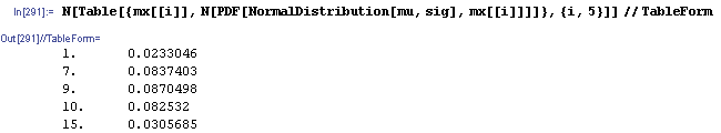
Let’s see this in an example:

Define the data set mx: 
mx={1,7,9,10,15}

Calculate the optimal mu and sigma:
dN=Length[mx];
mu=Sum[mx[[i]]/dN,{i,1,dN}];
sig =Sqrt[Sum[(mx[[i]]-mu)^2,{i,1,dN}]/dN];
Print["mu = ",N[mu]];
Print["sigma = ",N[sig]];

Now, let’s see this Gaussian Distribution Function:
<<Statistics`NormalDistribution`
ndist=NormalDistribution[mu,sig];

Clustering (or grouping) items using a defined similarity of selected properties is an effective way to classify the data, but also (and probably more important) aspect of clustering is to pick up abnormal pieces that are different from the other clusterable "herd". These exceptions may be the ones that we’re looking (or unlooking) for!

There is this simple clustering method called K-means Clustering. Suppose that you have N particles (atoms/people/books/shapes) defined by 3 properties (coordinates/{height, weight, eye color}/{title,number of sold copies,price}/{number of sides,color,size}). You want to classify them into K groups. A way of doing this involves the K-means Clustering algorithm. I have listed some examples to various items & their properties, but from now on, for clarity and easy visionalizing, I will stick to the first one (atoms with 3 coordinates, and while we’re at it, let’s take the coordinates as Cartesian coordinates).

The algorithm is simple: You introduce K means into the midst of the N items. Then apply the distance criteria for each means upon the data and relate the item to the nearest mean to it. Store this relations between the means and the items using a responsibility list (array, vector) for each means of size (dimension) N (number of items).

Let’s define some notation at this point:

• Designate the position of the k^th mean by m_k.
• Designate the position of the j^th item by x_j.
• Designate the responsibility list of the k^th mean by r_k such that the responsibility between that k^th mean and the j^th item is stored in the j^th element of r_k. If  r_k[j] is equal to 1, then it means that this mean is the closest mean to the item and 0 means that, some other mean is closer to this item so, it is not included in this mean’s responsibility.

The algorithm can be built in 3 steps:

0. Ä°nitialize the means. (Randomly or well calculated)

1. Analyze: Check the distances between the means and the items. Assign the items to their nearest mean’s responsibility list.

2. Move: Move the means to the center of mass of the items each is responsible for. (If a mean has no item it is responsible for, then just leave it where it is.)

3. Check: If one or more mean’s position has changed, then go to 1, if not exit.

That’s all about it. I have written a C++ code for this algorithm. It employs an object called kmean (can you guess what it is for? ) which has the properties and methods as:

class kmean
{
 private:
  unsigned int id,n;//"id" is for the unique identifier and "n" is the total number of items in the world.
  double x,y,z;//coordinates of the mean
  gsl_vector * r;//responsibility list of the mean
  char buffer [150];//some dummy variable to use in the "whereis" method
  unsigned int r_tott;//total number of data points this mean is responsible for

 public:
  kmean(int ID,double X, double Y, double Z,unsigned int N);
  ~kmean();
  //kmean self(void);
  int move(double X, double Y, double Z);//moves the mean to the point(X,Y,Z)
  int calculate_distances(gsl_matrix *MatrixIN, int N, gsl_matrix *distances);//calculates the distances of the "N" items with their positions defined in "MatrixIN" and writes these values to the "distances" matrix
  char * whereis(void);//returns the position of the mean in a formatted string
  double XX(void) {return x;}//returns the x-component of the mean’s position
  double YY(void) {return y;}//returns the y-component of the mean’s position
  double ZZ(void) {return z;}//returns the z-component of the mean’s position
  int II(void) {return id;}//returns the mean’s id
  int NN(void) {return n;}//returns the number of items in the world (as the mean knows it)
  int RR(void);//prints out the responsibility list (used for debugging purposes actually)
  gsl_vector * RRV(void) {return r;}//returns the responsibility list
  int set_r(int index, bool included);//sets the "index"th element of the responsibility list as the bool "included". (ie, registers the "index". item as whether it belongs or not belongs to the mean)
  int moveCoM(gsl_matrix *MatrixIN);//moves the mean to the center of mass of the items it is responsible for
  int RTOT(void) {return r_tott;}//returns the total number of items the mean is responsible for
  };
int check_distances(gsl_matrix* distances, int numberOfWorldElements, kmean **means);//checks the "distances" matrix elements for the means in the "means" array and registers each item in the responsibility list of the nearest mean.
double distance(double a1, double a2,double a3,double b1,double b2,double b3);//distance criteria is defined with this function

Now that we have the essential kmean object, the rest of the code is actually just details. Additionaly, I’ve included a random world generator (and by world, I mean N items and their 3 coordinates, don’t be misled). So essentialy, in the main code, we have the following lines for the analyze section:

  for (i=0;i<dK;i++)
   means[i]->calculate_distances(m,dN,distances);
  
  check_distances(distances,dN,means);

which first calculates the distances between each mean (defined as elements of the means[] array) and item (defined as the rows of the m matrice with dNx4 dimension (1st col: id, cols 2,3,4: coordinates) and writes the distances into the distances matrice (of dimensions dNxdK) via the calculate_distances(…) method. dN is the total number of items and dK is the total number of means. Then analyzes the distances matrice, finds the minimum of each row (because rows represent the items and columns represent the means) and registers the item as 1 in the nearest means’s responsibility list, and as 0 in the other means’ lists via the check_distances(…) method.

Then, the code executes its move section:

  for(i=0; i<dK; i++)
  {
   means[i]->moveCoM(m);
   […]
  }

which simply moves the means to the center of mass of the items they’re responsible for. This section is followed by the checkSufficiency section which simply decides if we should go for one more iteration or just call it quits.

  counter++;
  if(counter>=dMaxCounter) {f_maxed = true;goto finalize;}

  gsl_matrix_sub(prevMeanPositions,currMeanPositions);
  if(gsl_matrix_isnull(prevMeanPositions)) goto finalize;
  […]
  goto analyze;

as you can see, it checks for two things: whether a predefined iteration limit has been reached or, if at least one (two 😉 of the means moved in the last iteration. finalize is the section where some tidying up is processed (freeing up the memory, closing of the open files, etc…)

The code uses two external libraries: the Gnu Scientific Library (GSL) and the Templatized C++ Command Line Parser Library (TCLAP). While GSL is essential for the matrix operations and the structs I have intensely used, TCLAP is used for a practical and efficient solution considering the argument parsing. If you have enough reasons for reading this blog and this entry up to this line and (a tiny probability but, anyway) have not heard about GSL before, you MUST check it out. For TCLAP, I can say that, it has become a habit for me since it is very easy to use. About what it does, it enables you to enable the external variables that may be defined in the command execution even if you know nothing about argument parsing. I strictly recommend it (and thank to Michael E. Smoot again 8).

The program can be invoked with the following arguments:

D:\source\cpp\Kmeans>kmeans –help

USAGE:

   kmeans  -n <int> -k <int> [-s <unsigned long int>] [-o <output file>]
           [-m <int>] [-q] [–] [–version] [-h]

Where:

   -n <int>,  –numberofelements <int>
     (required)  total number of elements (required)

   -k <int>,  –numberofmeans <int>
     (required)  total number of means (required)

   -s <unsigned long int>,  –seed <unsigned long int>
     seed for random number generator (default: timer)

   -o <output file>,  –output <output file>
     output file basename (default: "temp")

   -m <int>,  –maxcounter <int>
     maximum number of steps allowed (default: 30)

   -q,  –quiet
     no output to screen is generated

   –,  –ignore_rest
     Ignores the rest of the labeled arguments following this flag.

   –version
     Displays version information and exits.

   -h,  –help
     Displays usage information and exits.

   K-Means by Emre S. Tasci, <…@tudelft.nl> 2007

 The code outputs various files:

<project-name>.means.txt : Coordinates of the means evolution in the iterations
<project-name>.meansfinal.txt : Final coordinates of the means
<project-name>.report : A summary of the process
<project-name>.world.dat : The "world" matrice in Mathematica Write format
<project-name>.world.txt : Coordinates of the items (ie, the "world" matrice in XYZ format)
<project-name>-mean-#-resp.txt : Coordinates of the items belonging to the #. mean

and one last remark to those who are not that much accustomed to coding in C++: Do not forget to include the "include" directories! 

Check the following command and modify it according to your directory locations (I do it in the Windows-way 🙂

g++ -o kmeans.exe kmeans.cpp -I c:\GnuWin32\include  -L c:\GnuWin32\lib -lgsl -lgslcblas -lm

(If you are not keen on modifying the code and your operating system is Windows, you also have the option to download the compiled binary from here)

The source files can be obtained from here.

And, the output of an example with 4000 items and 20 means can be obtained here, while the output of a tinier example with 100 items and 2 means can be obtained here.

I’m planning to continue with the soft version of the K-Means algorithm for the next time…

References: Information Theory, Inference, and Learning Algorithms by David MacKay

We’re soon going to need this information when playing a game called clustering so, it’s handy to have this around.

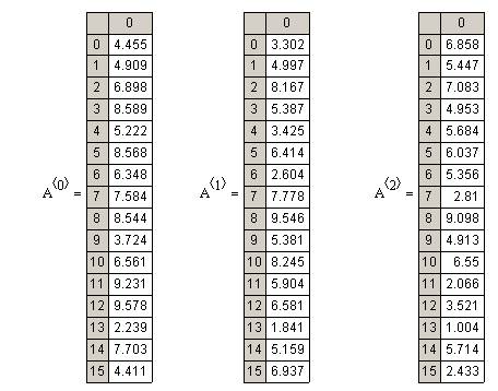
Suppose that the data belong to the positions of some number of particles given in Cartesian coordinates. The file (let’s assume it resides in the root of the d drive, having the name "lol1.txt") looks something similar to this:

 4.455  3.302  6.858 
 4.909  4.997  5.447 
 6.898  8.167  7.083 
 8.589  5.387  4.953 
 5.222  3.425  5.684 
 8.568  6.414  6.037 
 6.348  2.604  5.356 
 7.584  7.778  2.810 
 8.544  9.546  9.098 
 3.724  5.381  4.913 
 6.561  8.245  6.550 
 9.231  5.904  2.066 
 9.578  6.581  3.521 
 2.239  1.841  1.004 
 7.703  5.159  5.714 
 4.411  6.937  2.433 

First, let’s try it in Mathematica:

m=OpenRead["d:\lol1.txt"];
k= ReadList[m,Number];
Close[m];
(k =Partition[k,3]) // TableForm

(* And you can definitely Plot it too *)
<<Graphics`Graphics3D`
PlotStyle->{{PointSize[0.04],GrayLevel[0.09]}}]

Actually, I just copied the above code from a previous entry (but I had updated it just yesterday, so it is still fresh) the output graph will look like this:

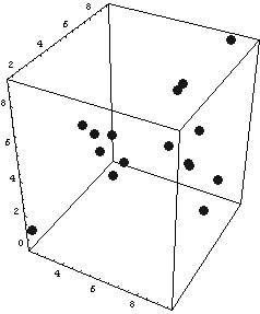
It is not that much practical to change the view angle (or most probably I don’t know how to do it) using Mathematica…

You can, for example, try something like this:
For[i=1,i<10,i+=1,ScatterPlot3D[k,PlotStyle->{{PointSize[0.04],GrayLevel[0.09]}},ViewPoint->{-2,i,2},AxesLabel->{"x","y","z"}]]

Or, if you have Mathcad with you, you can do this much simpler and more enjoyable way, too (but be warned, if I believed that Mathcad was superior to Mathematica, I would have a category for Mathcad instead of Mathematica category I’m having now – Mathcad actually from time to time makes you want to bite the keyboard! ;)! I decided to use Mathcad to visualize my scatter pattern and at once realized that, it has been nearly 5 years since I last used it. My favourite package used to be MapleV but -in my opinion- the Waterloo guys just tore it down when they switched the code language to Java. That was when our ways parted. Maple had nice graphics feature, too. So, if you’re using please send me your version of this entry… So, back to Mathcad:

First, from the "Insert…" menu, select "Component", then "File Read or Write" as the type and then select "Read from file". Browse to the designated file and make sure that "Use comma as decimal symbol" is unchecked since we’re using "." for the seperator. By the way, I’m using Mathcad2001 so it may (may?! more like surely!) be a little bit different about the options…

Attach a symbol to this file, say A so that now we have smt like:

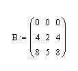
Now, just for the fun of it, define another set like:

You may also check your data if you want:

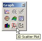
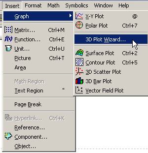
Now define a 3D Scatter Plot either from the Graph Pallette, or more preferably from the Insert menu:

Fill in the data section of the plot as (A^<0>,A^<1>,A^<2>),(B^<0>,B^<1>,B^<2>) and it’s all yours!

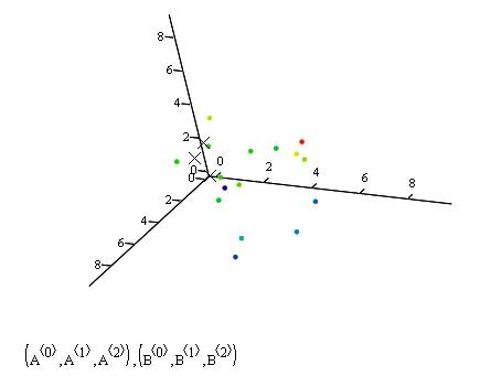
With mathcad I was able to rotate the graph whichever way I wanted and also could easily include data from different sources (like the A and B in the example) and plot them any way I wanted to. Here are the snapshots from a more "cute" plot with 500 data points:

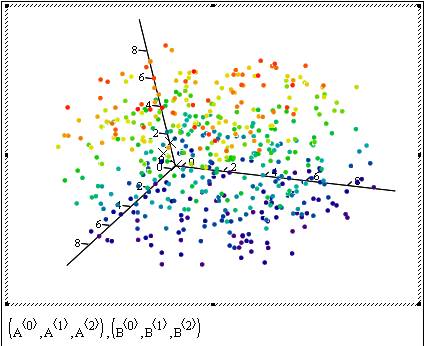
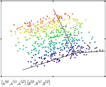
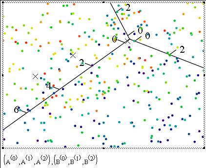
Hint for our game to be announced: Let’s call the little points in the plot as data’s and the Xs as "K-Means" 

Yesterday, I received great news from my dear former supervisor, Prof. Erkoç, that my Generation and Simulations of Nanostructures of Cage Structures titled Ph.D. thesis has been selected as one of the thesis of the year by METU Mustafa Parlar Foundation, the most distinctive and prestigious award a METU thesis can receive!

I would like to express my gratitude to Prof. Erkoç, all my friends and the physics department for the great days I’ve enjoyed for the seven years I was in METU. I will always cherish the memories… I hope, here in my new home S&C/MSE@TUDelft, I will live up to the expectations.

With Prof. Şakir Erkoç sitting in the front row, rest of our team is (from left to right):
O.Barış Malcıoğlu, Hande Üstünel, E. Deniz Çalışır Tekin, Nazım Dugan, Emre S. Taşcı, Rengin Peköz

Yesterday, I told my battalion-buddy, Andy about the pregnancy example and, he recalled another example, with the shuffling of the three cups and a ball in one of them. The situation is proposed like this:

The dealer puts the ball in one of the cups and shuffles it so fast that at one point you lose the track and absolutely have no idea which cup has the ball. So, you pick a cup randomly (let’s say the first cup) but for the moment, don’t look inside. At this point, the dealer says, he will remove one of the remaining two cups and he guarantees you that, the one he removes does not have the ball. He even bestows you the opportunity to change your mind and pick the other one if you like. The question is this: Should you

a) Stick to the one you’ve selected or,

b) Switch to the other one or,

c) (a) or (b) – what does it matter?

Today, while I was studying MacKay’s book Theory, Inference, and Learning Algorithms, I came upon to the same example and couldn’t refrain myself from including it on this blog.

First, let’s solve the problem with simple notation. Let’s say that, initially we have picked the first cup, the probability that this cup has the ball is 1/3. There are two possibilities: Whether in reality the 1st cup has the ball indeed, or not.

i) 1st cup has the ball (1/3 of all the times): With this situation, it doesn’t matter which of the two cups remaining is removed.

ii) 1st cup doesn’t have the ball (2/3 of all the times): This time, the dealer removes the one, and the remaining cup has the ball.

So, to summarize, left with the two cups, there’s a 1/3 probability that the ball is within the cup we have chosen in the beginning while there’s the 2/3 probability that the ball is within the other cup. So, switching is the advantegous (did I spell it correctly? Don’t think so.. ) / To put it in other words: option (b) must be preffered to option (a) and actually, option (c) is wrong.

Now, let’s compute the same thing with the formal notations:

Let H_i be define the situation that the ball is in cup i. D denotes the removed cup (either 2 or 3). Now, initially the ball can be in any of the three cups with equal probabilities so

Now, since we have selected the 1st cup, either 2nd or the 3rd cup will be removed. And we have three cases for the ball position:

The first column represents that the ball is in our selected cup, so it doesn’t matter which of the remaining cups the dealer will remove. Each of the remaining cup has the same probability to be removed which is 0.5. The second column is the situation when the ball is in the second cup. Since it is in the second cup, the dealer will be forced to remove the third cup (ie P(D=3|H₂)=1 ).Third column is similar to the second column.

Let’s suppose that, the dealer removed the third cup. With the 3rd cup removed, the probability that the ball is in the i. cup is given by: (remember that H_i represents the situation that the ball is in the i. cup)

for our purposes, P(D=3) is not relevant, because we are looking for the comparison of the first two probabilities (P(D=3) = 0.5, by the way since it is either D=2 or D=3).

meaning that it is 2 times more likely that the ball is in the other cup than the one we initially had selected.

Like John, Jo’s funny boyfriend in the previous bayesian example, used in context to show the unlikeliness of the "presumed" logical derivation, MacKay introduces the concept of one million cups instead of the three. Suppose you have selected one cup among the one million cups. Then, the dealer removes 999,998 cups and you’re left with the one you’ve initially chosen and the 432,238th cup. Would you now switch, or stick to the one you had chosen?